1 Introduction

Burgers' equations mostly appear in applied sciences such as fluid mechanics, mathematical modeling of turbulence, and approximate theory of flow via a shockwave travelling in a viscous fluid [1-3]. The one-dimensional coupled Burger equation is seen as a simple model of sedimentation and/or evolution of scaled volume concentrations of two types of particles in fluid suspensions and colloids under the effect of gravity. Several researchers have proposed analytical and numerical approaches for solving the one-dimensional Burger and coupled Burger equations. These approaches include the Variational Iteration Method (VIM), the Adomian Decomposition Method (ADM), the Homotopy Analysis Method (HAM), the Differential Transformation Method (DTM), the Reduced Differential Transform Method (RDTM), the modified extended tanh-function method, the Chebyshev spectral collocation method, and so on [4-12].

In general, the one-dimensional coupled nonlinear Burger equation of integer order is of the form:

\[u_{t} + \xi_{1}u_{xx} + \xi_{2}uu_{x} + \gamma(uv)_{x} = 0 v_{t} + \mu_{1}v_{xx} + \mu_{1}vv_{x} + \eta(uv)_{x} = 0\] (1)

subject to initial conditions (Eq. (2)) and the Dirichlet boundary conditions (Eq. (3)) as follows:

\[u(x,0) = g_1(x) v(x,0) = g_2(x)\] (2)

\[u(x,t) = h_1(x,t)\] \[v(x,t) = h_2(x,t)\] (3)

where \(x \in \Omega\) t > 0 for \(\Omega = \{x : x \in [c, d]\}\) as the computational domain while \(\xi_1, \xi_1, \mu_1\) and \(\mu_2\) are real constants, and \(\gamma\) and \(\eta\) are arbitrary constants that depend on the system's parameters.

In what follows, the extension of Eq. (1) to time-fractional order will be considered. Hence, the time-fractional coupled Burger equation (TFCBE) is of the form:

\[\text{[rumus tidak dapat ditampilkan dengan baik — lihat PDF asli]}\] \[(4)\]

Even though fractional derivatives (FDs) may appear old as a subject, they have received a remarkable interest in recent years for handling complex phenomena in applied sciences and engineering [13,14]. There are several types or forms of FDs, viz.: Caputo, Riemann-Liouville, Riesz, Weyl, Grunward, Coimbra, Canavati, Marcharud, Hadamard, Chen, Davidson-Essex, and Osler [15-17].

Recently, Yang [18], for the first time in the literature, has considered a class of FDs of constant and variable orders where the proposed formulas find vital expression in the description of fractional-order heat transfer equations in complex media. For recent work on LFOs, the reader is referred to [19] and the references therein. The notion of fractional Burger equations serves as a response for an expression that can be varied to describe the order of the derivative. In a generalized form, Momani [20] considered by means of ADM, the non-perturbation analytical solutions of the Burger's equation with timeand space-fractional orders. Yang, et al. [21] investigated a family of local fractional two-dimensional Burger-type equations by means of the local fractional Riccati differential equation method. Other reports on Burger equations include [22-25]. In the present work, we considered a onedimensional time-fractional coupled Burger equation of the form in Eq. (4) via a local fractional differential operator (LFDO) based on the MDTM for approximate-analytical solution. This method involves less computational work and requires less computational time.

2 Preliminaries and Notations on Fractional Calculus

In fractional calculus, the power of the differential operator is considered a real or complex number. Here, a brief introduction to fractional calculus will be given. For more notes and details regarding the definitions and properties of fractional calculus the reader is referred to [14-17, 26-28].

Suppose \(D = d'(\cdot)\) and J are differential and integral operators respectively. Then the following definitions hold:

Definition (a): Let \(\ell(x)\), x > 0 be a real function, then \(\ell(x)\) is said to belong to the space \(\overline{C}_v\), \(v \in \mathbb{R}\) if there exists \(\lambda \in \mathbb{R}\) (\(\lambda > v\)) such that \(\ell(x) = x^{\lambda} \ell(x)\) where \(\ell_1(x) \in \overline{C}(0,\infty)\). In addition, \(\ell(x)\) is said to be in the space \(\overline{C}_v^{\xi}\) if and only if \(\ell^{\xi} \in \overline{C}_v^{\xi}\), \(\xi \in \mathbb{N}\).

Definition (b): The Riemann-Liouville (R-L) fractional integration of \(\ell(x)\) of order \(\alpha \ge 0\), for \(\ell \in C_v\), \(v \ge -1\) is:

\[\begin{cases} J^{\alpha}\ell(x) = (J^{\alpha}\ell)(x) = \frac{1}{\Gamma(\alpha)} \int_{0}^{x} (x-s)^{\alpha-1}\ell(s)ds, & \alpha > 0, \\ J^{0}\ell(x) = \ell(x), & x > 0. \end{cases}\] (5)

Definition (c): The R-L fractional derivative of \(\ell(x)\) is:

\[D^{\alpha}\ell(x) = \frac{d^{\phi}\left(J^{\phi-\alpha}\ell(x)\right)}{dx^{\phi}}.\] (6)

Definition (d): The Caputo fractional derivative (CFD) of \(\ell(x)\) is:

\[D^{\alpha}\ell(x) = \frac{J^{\phi-\alpha}\left(d^{\phi}\ell(x)\right)}{dx^{\phi}}, \ \phi-1 < \alpha < \phi, \ \phi \in \mathbb{N}.\] (7)

Note: the link between the R-L operator and the Caputo fractional differential operator is:

\[\left(J^{\alpha}D_{t}^{\alpha}\right)\ell(t) = \left(D_{t}^{-\alpha}D_{t}^{\alpha}\right)\ell(t)\] \[= \ell(t) - \sum_{k=0}^{n-1} \ell^{k}(0)\frac{t^{k}}{k!}, n-1 < \alpha < n, n \in \mathbb{N}\] (8)

As such,

\[\ell(t) = \left(J^{\alpha} D_{t}^{\alpha}\right) \ell(t) + \sum_{k=0}^{n-1} \ell^{k}(0) \frac{t^{k}}{k!}.\] (9)

Definition (e): The Mittag-Leffler (M-L) function

The M-L function, \(E_{\alpha}(z)\), is defined and denoted by the series representation as:

\[E_{\alpha}(z) = \sum_{k=0}^{\infty} \frac{z^{k}}{\Gamma(1+\alpha k)}, \quad \alpha \ge 0, \ z \in \mathbb{C}.\] (10)

Remark. For \(\alpha = 1\), \(E_{\alpha}(z)\) in Eq. (10) becomes:

\[E_{\alpha=1}(z) = e^z. (11)\]

3 Analysis of Zhou's Method (DTM)

Zhou's method [29], as remarked by many researchers in the literature, has been proven to be easier and simpler in terms of application for both linear and nonlinear differential models because it converts the said problems to their equivalents in algebraic recursive form, but this is not so when compared with other semi-analytical techniques, say VIM, ADM, HAM, and so on. DTM has received outstanding modifications for handling models of nonlinear types [30-33].

3.1 Overview of Zhou's Method (DTM)

For an analytic function, h(x) defined in a domain D, the differential transform (DF) of h(x) is defined and denoted by:

\[H(p) = \frac{1}{p!} \left[ \frac{d^p h(x)}{dx^p} \right]_{x=x_+}, \tag{12}\] and as such:

\[h(x) = \sum_{p=0}^{\infty} H(p)(x - x_{+})^{p}.\] (13)

Eq. (13) is referred to as the differential inverse transform (DIT) of H(p), where h(x) and H(p) are the original and the transformed functions respectively.

3.2 Basic properties (P1-P4) of the Solution Method [31, 34]

P1: If \[h(x) = \alpha h_a(x) \pm \beta h_b(x)\], then \(H(p) = \alpha H_a(p) \pm \beta H_b(p)\).

P2: If \[h(x) = \frac{\alpha d^{\eta} h_{+}(x)}{dx^{\eta}}\], \(\eta \in \mathbb{N}\), then \(H(p) = \frac{\alpha (p+\eta)!}{p!} H_{+}(p+\eta)\).

P3: If \[h(x) = h_{+}^{2}(x)\], then \(H(p) = \sum_{n=0}^{p} H_{+}(n)H_{+}(p-\eta)\).

P4: (Modified DTM of a fractional derivative)

If, \(f(x) = D_x^{\alpha} h(x)\) then

\[\Gamma\left(1 + \frac{p}{q}\right)F\left(p\right) = \Gamma\left(1 + \alpha + \frac{p}{q}\right)H\left(p + \alpha q\right). \tag{14}\]

Setting \(\alpha q = 1\) in Eq. (14) gives:

\[H(p+1) = \frac{\Gamma(1+\alpha p)}{\Gamma(1+\alpha(1+p))} F(p). \tag{15}\]

As such, for h(x), \(\alpha\)-analytic at \(x_0 = 0\),

\[h(x) = \sum_{\eta=0}^{\infty} H(\eta) x^{\frac{\eta}{q}} = \sum_{\eta=0}^{\infty} H(\eta) x^{\alpha\eta}.\] (16)

3.3 Analysis of the Fractional DTM

Consider the nonlinear fractional differential equation (NLFDE):

\[D_x^{\alpha} h(x) + L_{\{x\}} h(x) + N_{\{x\}} h(x) = q_+(x), h(x,0) = g_+(x), x > 0\] (17)

where \(D_x^{\alpha} = \frac{d^{\alpha}}{dt^{\alpha}}\) is the fractional Caputo derivative of h = h(x), whose projected differential transform is H(p), while \(L_{\{\cdot\}}\) and \(N_{\{\cdot\}}\) are differential operators (with respect to x) of linear and nonlinear type respectively, and \(q_+ = q_+(x)\) is the source term.

We rewrite Eq. (17) as:

\[\begin{cases} D_x^{\alpha} h(x) = -L_{\{x\}} h(x) - N_{\{x\}} h(x) q_+(x), h(0) = g_+(x) \\ \eta - 1 < \alpha < \eta, \eta \in \mathbb{N}. \end{cases}\] (18)

Applying the inverse fractional Caputo derivative, \(D_x^{-\alpha}\), to both sides of Eq. (18) and with regard to Eq. (8) gives:

\[h(x) = g(x) + D_x^{-\alpha} \left[ -L_{|x|} h(x) - N_{|x|} h(x) + q(x) \right], \ h(0) = g(x). \tag{19}\]

Thus, when w(x) is expanded in terms of fractional power series, the inverse projected differential transform of H(p) is given as follows:

\[h(x) = \sum_{n=0}^{\infty} H(\eta) x^{\alpha \eta} = w(0) + \sum_{n=1}^{\infty} H(\eta) x^{\alpha \eta} , w(x,0) = g_{+}(x) .\] (20)

4 Illustrative Applications

In this subsection, the proposed method is applied to an example of a coupled Burger equation of time-fractional order as follows:

Case Example: Consider the TFCBE of the form Eq. (4) with \(\xi_1 = -1\), \(\xi_2 = -2\), \(\mu_1 = -1\), \(\mu_2 = -2\) & \(\gamma = \eta = 1\). Thus yielding:

\[u_t^{\alpha} - u_{xx} - 2uu_x + (uv)_x = 0\] \[v_t^{\alpha} - v_{xx} - 2vv_x + (uv)_x = 0\] (21)

subject to:

\[u(x,0) = \sin x = v(x,0)\]. (22)

Solution Procedure:

Taking the LFDT of Eq. (21) gives:

\[LFDT\Big[u_t^{\alpha}-u_{xx}-2uu_x+(uv)_x=0\Big],\]

\[LFDT \left[ v_t^{\alpha} - v_{xx} - 2vv_x + (uv)_x = 0 \right].\]

Therefore,

\[\frac{\Gamma(1+\alpha(1+k))}{\Gamma(1+\alpha k)}U_{1+k} = U''_{x,k} + 2\sum_{r=0}^{k} U_{x,r}U'_{x,k-r} - \frac{\partial}{\partial x}\sum_{r=0}^{k} U_{r}V_{k-r}, \qquad (23)\]

\[\frac{\Gamma(1+\alpha(1+k))}{\Gamma(1+\alpha k)}V_{1+k} = V_{x,k}'' + 2\sum_{r=0}^{k} V_{x,r}V_{x,k-r}' - \frac{\partial}{\partial x}\sum_{r=0}^{k} U_rV_{k-r}.\] \[(24)\]

In recurrence form we have:

\[U_{k+1} = \frac{\Gamma(1+\alpha k)}{\Gamma(1+\alpha(1+k))} \left( U_{x,k}'' + 2\sum_{r=0}^{k} U_{x,r} U_{x,k-r}' - \frac{\partial}{\partial x} \sum_{r=0}^{k} U_{r} V_{k-r} \right), \tag{25}\]

\[V_{k+1} = \frac{\Gamma(1+\alpha k)}{\Gamma(1+\alpha(1+k))} \left( V_{x,k}'' + 2\sum_{r=0}^{k} V_{x,r} V_{x,k-r}' - \frac{\partial}{\partial x} \sum_{r=0}^{k} U_r V_{k-r} \right).\] (26)

Thus, for k = 0, k = 1, k = 2, k = 3, k = 4, k = 5 ..., we have respectively \((U_1, U_2, U_3, U_4, ...)\) and \((V_1, V_2, V_3, V_4, ...)\) as follows:

\[U_{1} = \frac{\Gamma(1)}{\Gamma(1+\alpha)} \left( U_{x,0}'' + 2\sum_{r=0}^{0} U_{x,r} U_{x,-r}' - \frac{\partial}{\partial x} \sum_{r=0}^{0} U_{r} V_{-r} \right)\] \[= \frac{1}{\Gamma(1+\alpha)} \left( U_{0}'' + 2U_{0} U_{x,0}' - \left( U_{0} V_{0} \right)' \right), \tag{27}\]

\[V_{1} = \frac{\Gamma(1)}{\Gamma(1+\alpha)} \left( V_{0}'' + 2 \sum_{r=0}^{0} V_{x,r} V_{x,-r}' - \frac{\partial}{\partial x} \sum_{r=0}^{0} U_{r} V_{-r} \right)\]

\[= \frac{1}{\Gamma(1+\alpha)} \left( V_0'' + 2V_0 V_0' - \left( U_0 V_0 \right)' \right), \tag{28}\]

\[U_{2} = \frac{\Gamma(1+\alpha)}{\Gamma(1+2\alpha)} \left( U_{1}'' + 2\left(U_{0}U_{1}' + U_{1}U_{0}'\right) - \left(U_{0}V_{1} + U_{1}V_{0}\right)'\right),\tag{29}\]

\[V_{2} = \frac{\Gamma(1+\alpha)}{\Gamma(1+2\alpha)} \left( V_{1}'' + 2(V_{0}V_{1}' + V_{1}V_{0}') - (U_{0}V_{1} + U_{1}V_{0})' \right), \tag{30}\]

\[U_{3} = \frac{\Gamma(1+2\alpha)}{\Gamma(1+3\alpha)} \left( U_{2}'' + 2\left(U_{0}U_{2}' + U_{1}U_{1}' + U_{2}U_{0}'\right) - \left(U_{0}V_{2} + U_{1}V_{1} + U_{2}V_{0}\right)' \right), \quad (31)\]

\[V_{3} = \frac{\Gamma(1+2\alpha)}{\Gamma(1+3\alpha)} \left( V_{2}'' + 2\left(V_{0}V_{2}' + V_{1}V_{1}' + V_{2}V_{0}'\right) - \left(U_{0}V_{2} + U_{1}V_{1} + U_{2}V_{0}\right)' \right), \tag{32}\] and so on.

Hence, using the initial condition: u(x, 0) = sinx = v(x, 0) with respect to the LFTM we obtain:

\[\begin{cases} U_{0} = V_{0} = \sin x, \ U_{2} = \frac{\sin x}{\Gamma(1+2\alpha)} = V_{2}, \ U_{4} = \frac{-\sin x}{\Gamma(1+4\alpha)} = V_{4}, \cdots \\ U_{1} = \frac{-\sin x}{\Gamma(1+\alpha)} = V_{1}, \ U_{3} = \frac{-\sin x}{\Gamma(1+3\alpha)} = V_{3}, \ U_{5} = \frac{-\sin x}{\Gamma(1+5\alpha)} = V_{5}, \cdots \end{cases}\](33)

Hence,

\[u(x,t) = \sum_{h=0}^{\infty} U_h t^{\alpha h}\] \[= \sin x - \frac{\sin x}{\Gamma(1+\alpha)} t^{\alpha} + \frac{\sin x}{\Gamma(1+2\alpha)} t^{2\alpha} - \frac{\sin x}{\Gamma(1+3\alpha)} t^{3\alpha} + \cdots\] \[= \sin x \left( 1 - \frac{t^{\alpha}}{\Gamma(1+\alpha)} + \frac{t^{2\alpha}}{\Gamma(1+2\alpha)} - \frac{t^{3\alpha}}{\Gamma(1+3\alpha)} + \cdots \right)\] \[= \sin x \sum_{n=0}^{\infty} \frac{(-1)^n t^{n\alpha}}{\Gamma(1+n\alpha)}.\] (34)

Similarly,

\[v(x,t) = \sum_{h=0}^{\infty} V_h t^{\alpha h} = \sin x \sum_{n=0}^{\infty} \frac{\left(-1\right)^n t^{n\alpha}}{\Gamma(1+n\alpha)}.\] (35)

Note: when \(\alpha = 1\), we have \(u(x,t) = \sin(x) \exp(-t) = v(x,t)\), which corresponds to the exact solution of the coupled Burger equation as contained in [1,4,35]. The exact and approximate solutions are presented graphically in Figure 1 through Figure 3.

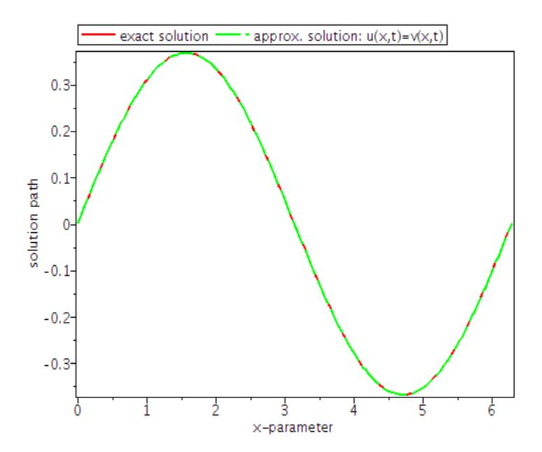
Figure 1 The solution graphs for t = 1 at \(\alpha = 1\).

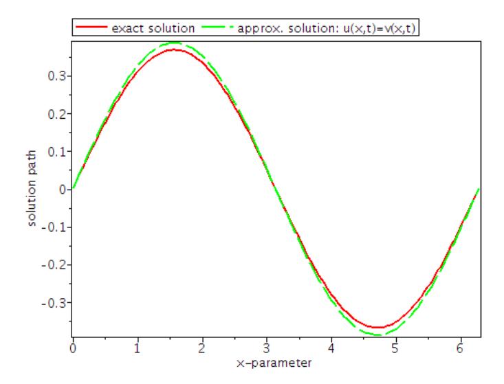
Figure 2 The solution graphs for ݐൌ1 at ߙ ൌ 0.8.

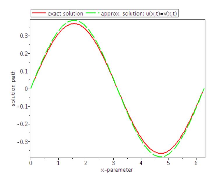
Figure 3 The solution graphs for ݐൌ1 at ߙ ൌ 0.8.

5 Concluding Remarks

We have successfully considered the approximate-analytic solutions of a system of time-fractional coupled Burger equations by means of a local fractional

operator (LFO) in the sense of the Caputo derivative. To demonstrate the effectiveness and robustness of the present technique, we used some illustrative examples; the solutions are provided in the form of convergent series. The method was shown to be efficient and reliable as it does not depend upon any process of identifying Lagrange multipliers, unlike the variational iteration method, even while still maintaining high-level accuracy. The method is therefore recommended for solving linear and nonlinear time-fractional differential equations (TFDEs) in other areas of applied science.

Acknowledgement

The authors are indeed grateful to Covenant University for their financial support and provision of a good working environment. They also wish to thank the anonymous reviewers for their productive remarks.