

1 Introduction
Systems of linear equations (SLEs) are ubiquitous in science and engineering applications. There are several approaches for solving them, broadly classified as direct and iterative methods. There are two general classes of iterative methods to solve SLEs: stationary and non-stationary methods. Stationary methods include Richardson [1], Jacobi, Gauss-Seidel [2], and Successive Over-relaxation (SOR) [3], among others. Non-stationary methods include
Received May 16th, 2017, 1st Revision October 24th, 2017, 2nd Revision February 17th, 2018, Accepted for publication March 6th, 2018.
Copyright © 2018 Published by ITB Journal Publisher, ISSN: 2337-5760, DOI: 10.5614/j.math.fund.sci.2018.50.2.4
Conjugate Gradient [4], BCG, BICG [5], GMRES, Arnoldi type [6], and Lanczos type [7,8]. Non-stationary methods are generally more efficient and suitable for large systems of linear equations. They are based on orthogonal polynomials and are often referred to as Krylov subspace methods [9,10].
Among the iterative methods, for solving large linear systems with a sparse non-symmetric matrix, those based on the Lanczos process are the most effective. This is because they feature short recurrence relations for the generation of the Krylov subspace, which means low cost and low memory requirement [5]. They are, however, prone to breakdown [11]. Ways to avoid breakdown in Krylov subspace algorithms have been researched extensively in the last decades, resulting in new, more robust and efficient algorithms using, for instance, restarting and switching strategies that allow us to restart and switch between Lanczos-type algorithms before they break down [12,13]. A recent work, discussed in Maharani & Salhi [14], considered three quality points for restarting Lanczos-types algorithms.
In this study, we propose a novel strategy for SLEs that have a unique solution, which takes advantage of the existence of patterns in the solutions generated by Lanczos-type algorithms. The patterns persist in the entries of the iterates during the iteration process. Interpolating every entry of the iterates allows to obtain model functions that can be used to predict the entries of a new iterate. This iterate is expected to be better than the previous iterates generated by the Lanczos-type algorithm.
This paper is organized as follows. In Section 1, we look at the background theory of Lanczos-type algorithms for solving SLEs. The motivation and derivation of the new approach are given in Sections 2 and 3, respectively. Section 4 discusses the numerical results of EIEMLA's implementation of algorithms A13/B6 and A13/B13. The conclusion is given in Section 5.
2 Review of Lanczos-type Algorithms for the Solution of SLEs
The Lanczos method to solve system
\[A\mathbf{x} = \mathbf{b} \,, \tag{1}\] where ∈௫ and vectors , ∈ , is based on the Krylov subspace method. If and are two Krylov subspaces in , then we can choose an initial approximate solution so that
\[\mathbf{x}_{k} - \mathbf{x}_{0} \in K_{k}(A, \mathbf{r}_{0}) \tag{2}\] and
\[\mathbf{r}_{k} = \mathbf{b} - \mathbf{x}_{k} \perp L_{k} = K_{k}(A^{T}, \mathbf{y})\] (3)
where \(\mathbf{r}_0 = \mathbf{b} - \mathbf{x}_0\) is the corresponding residual vector, and \(\mathbf{y}\) is an arbitrary non-zero vector. Moreover, the residual \(\mathbf{r}_k\) satisfies the condition:
\[\langle \mathbf{y}, A^i P_k(A) \mathbf{r}_0 \rangle = 0\], for \(i = 0, 1, ..., n-1\), (4)
where \(P_k(t) = 1 + \alpha_1 t + \dots + \alpha_k t^k\) is a residual polynomial, i.e. \((\mathbf{r}_k = P_k(A)\mathbf{r}_0)\), of degree k at most. This polynomial satisfies the normal condition, \(P_k(0) = 1\). Let c be a linear functional in the vector space of polynomials, defined by
\[c_i = c(\mathbf{x}^i) \tag{5}\]
If we set \(c_i = \langle \mathbf{y}, A^i \mathbf{r}_0 \rangle\), then Relation in Eq. (4) can be written as
\[c(t^{i}P_{k}(t)) = 0, i = 0, 1, ..., k-1\] (6)
Relation in Eq. (6) indicates that the highest degree of \(P_k\) is k, and it belongs to the family of orthogonal polynomials with respect to function c. Thus, by using formula \(\mathbf{r}_k = P_k(A)\mathbf{r}_0\), we can set up the update solution, which is \(\mathbf{x}_k = \mathbf{b} - A\mathbf{r}_k\). All of this is derived recursively.
Some formulas that Lanczos-type algorithms are based on have been discovered by Brezinski, et al. (see [15,16]). They include formulas \(A_i\) and \(B_j\), for i,j=1,2,...,10. The extension of these formulas, which involve polynomials with a difference in degrees of at most two or three, were investigated in Farooq & Salhi [17]. They are formulas \(A_i\) and \(B_j\), for i,j=11,12,...,16. New variants of the Lanczos-type algorithm, which combine Baheux-type and Farooq-type algorithms, have been investigated in Ulah, et al. [18] and Suharto, et al. [19], who discovered formulas , A13/B6 and A13/B10.
3 Motivation
Breakdown can be avoided in a variety of ways. Here, we suggest regression as a means for that purpose. When breakdown occurs it is possible to remove the last iterate that caused breakdown from the sequence of Lanczos-type algorithm points, regress on this sequence (their entries) to find a suitable model, and then use this model to generate new points that are within the sequence of points that would have been generated by the Lanczos-type algorithm if breakdown had not occurred.
The idea is to exploit patterns that may exist in the sequences generated by a given Lanczos-type algorithm. After running such an algorithm for a certain number of iterations it was pre-emptively stopped before it breaks down. We then considered the generated iterates to see if any patterns existed. To illustrate what we mentioned above, we considered a Lanczos-type algorithm such as Orthodir [15], and ran it for 30 iterations to solve an SLE in 50 dimensions. We collected all iterates and saved them in Eq. (7) as follows:
\[data_{sol} = \begin{bmatrix} x_1^{(1)} & x_1^{(2)} & \dots & x_1^{(50)} \\ x_2^{(1)} & x_2^{(2)} & \dots & x_2^{(50)} \\ \vdots & & & & \\ x_{30}^{(1)} & x_{30}^{(2)} & \dots & x_{30}^{(50)} \end{bmatrix}\] \[(7)\]
We then plotted all the above iterates by using the Parallel Coordinate System (PCS) [20-23]. By visualizing high-dimensional data, PCS gives insight into the behavior of high-dimensional iterates generated over a number of iterations. This is the main motivation behind our idea to exploit patterns that may exist in iterates generated by Lanczos-type algorithms to improve the robustness of these algorithms.
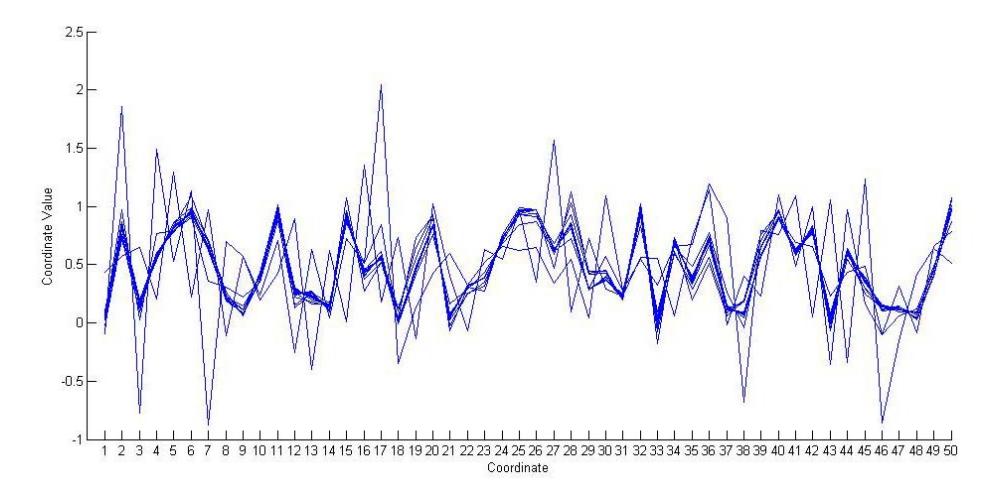
Figure 1 Behavior of EIEM Orthodir and Orthodir algorithms on SLEs in 50 dimensions. The blue line corresponding to EIEM Orthodir, has some very good points and grows much slower than the one corresponding to Orthodir.
Figure 1 illustrates the PCS representation of all iterates generated by Orthodir. The entries of the iterates are represented on the x-axis, while the values of the entries are represented on the y-axis. As we can see here, after some time several iterates start to form similar shapes. Our assumption is that these iterates are close enough to the true solution. In other words, these iterates have a small
residual norm. We investigated this further by exploiting the patterns at the level of a single coordinate. More precisely, we were interested in the patterns of the entries of the iterates. This allowed us to work in a single dimension. If we have k iterates of an n-dimension problem, the following sequence
\[S = \left\{ \mathbf{x}_1, \mathbf{x}_2, ..., \mathbf{x}_k \right\} \tag{8}\]
holds them all. Now, consider the first entries of all iterates in S, the second entries of all iterates in S, etc. A regression model over all first entries will be used to generate the 1st entry of a new point; a regression model over all 2<sup>nd</sup> entries will be used to generate the second entry of the new point, etc. In this fashion we generate a new point that, as we will establish later, belongs to the sequence of iterates of the Lanczos-type algorithm that was stopped prematurely according to some norm. This idea should be applicable for instance when Lanczos process-based algorithms are used to generate eigenvalues and eigenvectors and in any iterative process where breakdown is an issue.
4 Generating the Approximate Solutions Using Interpolation and Extrapolation Model
A new approach to enhance the stability of Lanczos-type algorithms was developed, henceforth called Embedded Interpolation and Extrapolation Model in Lanczos-type Algorithms (EIEMLA).
4.1 Derivation of EIEMLA
Consider k iterates that form set S as in Eq. (8). As explained above, among the \(\mathbf{x}_k\), there are some iterates with small residual norms in interval [m-j,k]. Let \(\mathbf{x}_m\) have a corresponding minimum residual norm, \(\|\mathbf{r}_m\|\) and set
\[V_1 = \left\{ \mathbf{x}_{m-j}, \mathbf{x}_{m-j+1}, \dots, \mathbf{x}_k \right\} \tag{9}\] where
\[\mathbf{x}_{m-j} = [x_{m-j}^{(1)}, x_{m-j}^{(2)}, \cdots, x_{m-j}^{(n)}]^{T}\] \[\mathbf{x}_{m-j+1} = [x_{m-j+1}^{(1)}, x_{m-j+1}^{(2)}, \cdots, x_{m-j+1}^{(n)}]^{T}\] \[\vdots\] \[\mathbf{x}_{k} = [x_{k}^{(1)}, x_{k}^{(2)}, \cdots, x_{k}^{(n)}]^{T}\] (10)
We assume that the sequences \(v_1 = \{x_{m-j}^{(1)}, x_{m-j+1}^{(1)}, \cdots, x_k^{(1)}\},\) \(v_2 = \{x_{m-j}^{(2)}, x_{m-j+1}^{(2)}, \cdots, x_k^{(2)}\},\) ..., and \(v_n = \{x_{m-j}^{(n)}, x_{m-j+1}^{(n)}, \cdots, x_k^{(n)}\}\) have special properties, such as increasing or decreasing monotonically. In this case,
\(v_1, v_2, ..., v_n\) are obtained by rearranging entries in Eq. (10). According to [24], each \(v_i\) for i = 1, 2, ..., n, is monotonic and convergent to its limit. This means that
\[\lim_{k \to \infty} x_k^{(i)} = x_i^* \tag{11}\]
If we set
\[w_{1} = \left\{ \left( t_{m-j}, \mathbf{x}_{m-j}^{(1)} \right), \left( t_{m-j+1}, \mathbf{x}_{m-j+1}^{(1)} \right), \dots, \left( t_{k}, \mathbf{x}_{k}^{(1)} \right) \right\}\] \[w_{2} = \left\{ \left( t_{m-j}, \mathbf{x}_{m-j}^{(2)} \right), \left( t_{m-j+1}, \mathbf{x}_{m-j+1}^{(2)} \right), \dots, \left( t_{k}, \mathbf{x}_{k}^{(2)} \right) \right\},\] \[\vdots\] \[w_{n} = \left\{ \left( t_{m-j}, \mathbf{x}_{m-j}^{(n)} \right), \left( t_{m-j+1}, \mathbf{x}_{m-j+1}^{(n)} \right), \dots, \left( t_{k}, \mathbf{x}_{k}^{(n)} \right) \right\}\] \[(12)\] where \(t \in R\), then we can use PCHIP to interpolate and extrapolate Eq. (12). Let \(f_i\), for i = 1, 2, ..., n, be functions of the interpolation process. This means they satisfy
\[f_i(t) \cong x_t^{(i)}\], for \(i = 1, 2, ..., n\), (13)
for some t = m - j, m - j + 1, ..., k. For \(t^* \in [k+1, s] \subset R\), we have
\[f_i(t^*) \cong x_r^{(i)}\], for \(i = 1, 2, ..., n\) (14)
where \(s \ge k+1\). It is guaranteed that \(x_r^{(i)}\) has a similar property as \(x_t^{(i)}\) since the later vectors are the extrapolation results of the first one. In fact, we use PCHIP to produce, \(x_t^{(i)}\), where it preserves the properties of the data and captures the persistent patterns of the data. This process terminates by rearranging vectors \(x_r\), with \(x_r^{(i)}\) being the \(i^{th}\) entries of the vector. This whole process is called Embedded Interpolation and Extrapolation Model in Lanczostype Algorithms (EIEMLA).
Theoretically, since PCHIP captures the persistent pattern of the \(i^{th}\) entry, i=1,2,...,n, of the iterates generated by a Lanczos-type algorithm, the entries of the new iterate, as a result of the model function, are likely to behave the same as those entries. Furthermore, we can produce as many vector solutions as we want by applying the functions \(f_i\) over \(t^* \in R\) without running the Lanczos-type algorithm again. However, we should be aware that the quality of these generated solutions may not be good enough, in which case we must either restart the iterative process from the best point or take the best solution found so far as the candidate solution. It is therefore, reasonable to choose the integer s
such that the residual norms of the iterates generated by these functions, \(\mathbf{x}_{k+1}, \mathbf{x}_{k+2}, \dots, \mathbf{x}_s\), are small enough. In this case, we obtain another sequence of the iterates generated by EIEMLA. It is expected that these iterates replace the 'missing' iterates not generated by the Lanczos-type algorithm due to breakdown.
4.2 Implementation of the EIEMLA Method
The above results suggest a procedure for EIEMLA (see Algorithm 1). As an illustration of the implementation of EIEMLA, consider System in Eq. (1) with n=5. Orthodir is used to solve it over 50 iterations. Following the above procedures, we first collect all of the 50 iterates as. \(S = \{\mathbf{x}_1, \mathbf{x}_2, ..., \mathbf{x}_{150}\}\). A visualization of several entries of S is shown in Figure 1, Section 1. Secondly, we calculate index m of iterate \(\mathbf{x}_m\) associated with the lowest residual norm, \(\|\mathbf{r}_m\|\). In this particular example, \(\|\mathbf{r}_m\| - 0.0067\) with m=17. Thus rearranging S as in Eq. (1) yields the following sequence:
\[w_{1} = \left\{ \left( t_{7}, \mathbf{x}_{7}^{(1)} \right), \left( t_{8}, \mathbf{x}_{8}^{(1)} \right), ..., \left( t_{50}, \mathbf{x}_{50}^{(1)} \right) \right\}\] \[w_{2} = \left\{ \left( t_{7}, \mathbf{x}_{7}^{(2)} \right), \left( t_{8}, \mathbf{x}_{8}^{(2)} \right), ..., \left( t_{50}, \mathbf{x}_{50}^{(2)} \right) \right\}\] \[w_{50} = \left\{ \left( t_{7}, \mathbf{x}_{7}^{(n)} \right), \left( t_{8}, \mathbf{x}_{8}^{(n)} \right), ..., \left( t_{50}, \mathbf{x}_{50}^{(n)} \right) \right\}\] \[(18)\] where t is an integer within the range [m-10,50]. The choice of this range is based on our observation that some good iterates can be found in it. Also, based on Figure 1, the entries of the iterates in that range are increasing or decreasing monotonically.
The next step is to interpolate each \(w_i\) in Eq. (18) using PCHIP to get functions \(f_i\). We use these functions to extrapolate and generate points that are outside the range. In this case, we choose \(t^* \in [17,50]\). The interpolation and extrapolation results are captured in Figure 2. As can be seen, PCHIP interpolates the data accurately and smoothly (see the blue curves). However, the extrapolation results in some points are of poor quality. In Figure 2(a), for instance, the blue curve, which represents the PCHIP data, goes up after the \(\{50\}^{th}\) iteration. The PCHIP curve, on the other hand, seems monotone after the \(\{50\}^{th}\) iteration in Figures 2(b), (2c), and (2d).
Among the iterates generated by Orthdir, some entries behave as in Figure 2(a). This means their trend goes up or down after k iterations. However, there are many other entries that behave monotonically. Since we put all entries in one vector, overall, the effect of the fluctuating entries is smaller, which means that a good approximate solution may be generated.
After calculating functions over ∗, we now have the approximate solutions as in Eq. (16). We compute the residual norms accordingly. The behavior of EIEM Orthodir and Orthodir for this case, is represented in Figure 3. As can be seen, generally, the residual norms of the iterates generated by EIEM Orthodir (the blue curve) are found below those generated by Orthodir (the red curve) from iteration 17 to 50. In fact, at iteration 31, the residual norm hits the value of 0.003. However, it goes up after iteration 71.
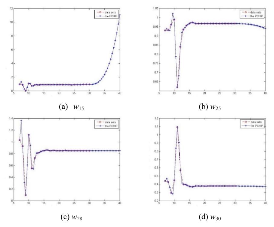
Figure 2 The interpolation and extrapolation results of sequences , for ൌ 7,8, … 50 as in Eq. (18). The red curve represents all of the entries of the ௧ sequence, while the blue curve represents their interpolation and extrapolation results using PCHIP.
We can safely say that some iterates generated by EIEM Orthodir have smaller residual norms than all previous iterates generated by the Orthodir. On its own, it does not find solutions with such low residual norms, even with a high number of iterations.
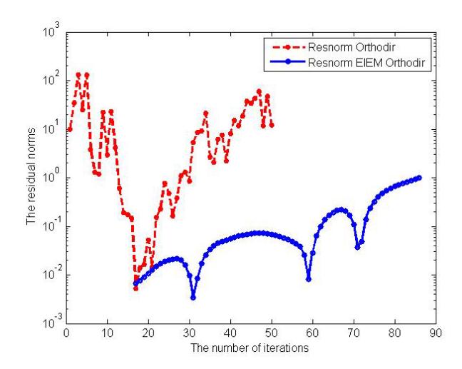
Figure 3 Behavior of EIEM Orthodir and Orthodir algorithms on SLEs in 50 dimensions. The blue line, corresponding to EIEM Orthodir, has some very good points and grows much slower than that corresponding to Orthodir.
Algorithm 1. The EIEMLA method
- 1. Initialization. Choose \(\mathbf{x}_0\) and \(\mathbf{y}\), Set \(\mathbf{r}_0 = \mathbf{b} A\mathbf{x}_0\), \(\mathbf{y}_0 = \mathbf{y}\), and \(\mathbf{z}_0 = \mathbf{r}_0\).
- 2. Fix the number of iterations to, say, k, and the tolerance, \(\epsilon\), to E-13 and run the Lanczos-type algorithm.
- 3. IF \(\{\|\mathbf{r}_m\| < \epsilon\}\)
- 4. The solution is obtained
- 5. Stop
- 6. ELSE
- 7. Collect all k vector solutions as in Eq. (7).
- 8. Choose some j such that m j < k.
- 9. Set \(w_i\) as in Eq. (18), for i = 1, 2, ..., n.
- 10. Interpolate \(w_i\) using PCHIP to get \(f_i\).
- 11. Choose \(t^* \in [m, s] \subset R\), where \(s \le m \le k\) is an integer, and calculate \(f_i(t^*)\)
- 12. FOR \(\{q = 1, 2, ..., l\}\) DO
- 13. Arrange vectors
14. \[\mathbf{x}_{*}^{(q)} = \begin{bmatrix} f_{1}^{(q)}(t^{*}) \\ f_{2}^{(q)}(t^{*}) \\ \vdots \\ f_{n}^{(q)}(t^{*}) \end{bmatrix}\] (16)
- 15. Where l = length([m, s]).
- 16. Calculate the residual norms of Eq. (16) as follows
17. \[\left\| \mathbf{r}_{*}^{(q)} \right\| = \mathbf{b} - A \mathbf{x}_{*}^{(q)}\] (17)
- 18. ENDFOR
- 19. ENDIF
- 20. The solutions of the systems are \(\left\{x_*^{(1)}, x_*^{(2)}, \dots, x_*^{(l)}\right\}\)
- 21. Stop.
4.3 Formal Basis of EIEMLA
As mentioned in the previous section, the sequences generated by Lanczos-type algorithms have the property of monotonicity. Since we consider PCHIP, which preserves monotonicity [25], to interpolate the sequences, we can assume that points returned by the function are also monotonic. This leads to the theorem below, which guarantees the monotonicity of sequences generated by Lanczos-type algorithms. The proofs of the theorems can be seen in the Appendix.
Theorem 1. Given a sequence \(x_k\) of k iterates generated by a Lanczos-type algorithm, sequences of \(x_k^{(i)}\), i = 1, 2, n, and k = 1, ... namely the entries of k iterates, are monotonic.
Lemma 1 [26]. Let \(A = VAV^{-1}\) be a nonsingular diagonalizable matrix, where V is a matrix that consists of the eigenvectors of A, S is a diagonal matrix with
\[A = \begin{bmatrix} B & -I & \cdots & \cdots & 0 \\ -I & B & -I & \cdots & & \\ \vdots & \ddots & \ddots & \ddots & \vdots \\ \vdots & & -I & B & -I \\ 0 & \cdots & \cdots & -I & B \end{bmatrix}\] \[a_{ii} \in \sigma(A) \text{ being the diagonal entries, and } \sigma(A)\] \[A = \begin{bmatrix} B & -I & \cdots & 0 \\ \vdots & \ddots & \ddots & \vdots \\ \vdots & & & & & & \\ 0 & \cdots & \cdots & & & & \\ \end{bmatrix}\] is the set of the eigenvalues of A. Then, \(||P_k(A)|| \le \kappa_2(V) \max_{\lambda \in \sigma(A)} |\lambda|\) where \(\kappa_2(V)\) is the condition of matrix V.
Theorem 2. Let \(x_1, x_2, ..., x_k, x_{k+1}\) be the iterates generated by the Orthodir algorithm. Let \(x_{model}\) be a vector returned by EIEMLA as explained in the previous section. Then, for some \(\in > 0\), \(||x_{k+1} - x_{model}|| \le \in\), where ||.|| is the Euclidean norm.
Based on the above theorem, we finally show that the residual norm of an iterate generated by EIEMLA is always smaller or equal to that of an iterate
generated by the Lanczos-type algorithm considered. In other words, better solutions are generated through this process.
Theorem 3. Let \(x_1, x_2, ..., x_k\) be the iterates generated by the Orthodir algorithm. Let \(r_{model}\) be a residual vector that corresponds to the iterate generated by EIEMLA. Then, \(||r_{model}|| \le (1 + |\lambda|) ||r_k||\).
5 Numerical Results and Discussion
Our test problems used in this study arise in the 5-point discretization of the operator \(-\frac{\partial^2}{\partial x^2} - \frac{\partial^2}{\partial y^2} + \gamma \frac{\partial}{\partial x}\) on a rectangular region [27]. This yields System in Eq. (1) with
\[A = \begin{bmatrix} B & -I & \cdots & \cdots & 0 \\ -I & B & -I & \cdots & & \\ \vdots & \ddots & \ddots & \ddots & \vdots \\ \vdots & & -I & B & -I \\ 0 & \cdots & \cdots & -I & B \end{bmatrix} \text{ and } B = \begin{bmatrix} 4 & \alpha & \cdots & \cdots & 0 \\ \beta & 4 & \alpha & \cdots & & \\ \vdots & \ddots & \ddots & \ddots & \vdots \\ \vdots & & \beta & 4 & \alpha \\ 0 & \cdots & \cdots & \beta & 4 \end{bmatrix}\] and \(\alpha = -1 + \delta\), \(\beta = -1 - \delta\), \(\delta\) takes values 0; 0.2; 0.5; 0.8; 5; 8. The parameter \(\delta\) plays an important role in the singularity of matrix A. For instance, when \(\delta = 0\), A is a symmetric matrix. The condition number of matrix A for this particular value of \(\delta\) is large enough, i.e. 119.9999. Any system built by this matrix tends to be ill-conditioned [28-30]. When \(\delta\) is large enough, matrix A can become well-conditioned. We can also say here that the SLEs that involve matrix A have a unique solution.
Furthermore, we use iterations \(k = 100 \le n\). The choice of k is based on the observation that Lanczos-type algorithms generally fail to find a good approximate solution after 100 iterations. In addition, the right-hand side \(\boldsymbol{b}\) is taken to be \(\boldsymbol{b} = A\boldsymbol{x}\), where \(\boldsymbol{x} = (x_1, x_2, ..., x_n)^T\) is the solution of the system, and \(x_i\), i = 1, 2, ..., n is a random value between 0 and 1. We use formulas \(A_{13}/B_6\) and \(A_{13}/B_{13}\) in this experiment as representative of Lanczos-type algorithms. Note, that the first formula is a new type of Lanczos algorithm, investigated in Ullah, et al. [18], while the second one is found in Suharto, et al. [19].
5.1 Numerical Results
The test problems were carried out under MATLAB 2015b on a computer with an Intel 2.40 GHz processor, Core i7, and 16 GB RAM. The aim of the experiment was to examine the reduction in the residual norm of the iterates generated by EIEMLA compared with the original Lanczos-type algorithms. All of the results are recorded in Tables 1 and 2, and visualized graphically.
Table 1 Comparison of residual norms of iterates generated by A13/B6 and generated by EIEM A13/B6 over 100 iterations.
| Dim n | A13B6 ‖𝐫𝒌‖ | EIEM A13B6 ‖𝐫𝒎𝒐𝒅𝒆𝒍‖ | Time (s) |
|---|---|---|---|
| 1000 | 3.62E+02 | 10.6498 | 0.3232 |
| 2000 | 6.42E+04 | 8.4998 | 0.3903 |
| 3000 | NaN | 4.9849 | 0.6783 |
| 4000 | 1.87E+09 | 12.3174 | 17.8791 |
| 5000 | 1.87E+09 | 12.3174 | 0.6783 |
| 6000 | NaN | 16.6164 | 0.7714 |
| 7000 | 4.69E+03 | 12.7736 | 0.8029 |
| 8000 | 5.03E+08 | 2.2334 | 1.0650 |
| 9000 | 3.54E+03 | 1.1718 | 0.9489 |
| 10000 | 9.56E+05 | 14.9270 | 1.0276 |
| 20000 | NaN | 9.6835 | 1.6685 |
| 30000 | 7.24E+10 | 152.9614 | 2.6506 |
| 40000 | 1.15E+03 | 13.1240 | 3.3747 |
| 50000 | 1.13E+10 | 53.2363 | 4.3543 |
| 60000 | 1.67E+06 | 154.0032 | 5.1728 |
| 70000 | NaN | 138.9045 | 5.8259 |
| 80000 | NaN | 82.3836 | 6.6018 |
| 90000 | 7.13E+03 | 23.2396 | 7.1726 |
| 100000 | 1.53E+07 | 4.4710 | 8.0383 |
Table 2 Comparison of residual norms of iterates generated by A13/B13 and generated by EIEM A13/B13 over 100 iterations.
| Dim n | A13B13 ‖𝐫𝒌‖ | EIEM A13B13 ‖𝐫𝒎𝒐𝒅𝒆𝒍‖ | Time (s) |
|---|---|---|---|
| 1000 | NaN | 7.0391 | 0.3607 |
| 2000 | NaN | 3.6217 | 0.4311 |
| 3000 | NaN | 57.3744 | 0.7274 |
| 4000 | NaN | 50.1365 | 1.0101 |
| 5000 | NaN | 40.5467 | 1.5103 |
| 6000 | NaN | 3.5261 | 2.0745 |
| 7000 | NaN | 29.2577 | 2.6821 |
| 8000 | NaN | 78.5510 | 2.9997 |
| 9000 | NaN | 713.7055 | 4.2056 |
| 10000 | NaN | 9.9809 | 4.9926 |
| 20000 | NaN | 19.6627 | 20.0117 |
| 30000 | NaN | 24.7834 | 54.4602 |
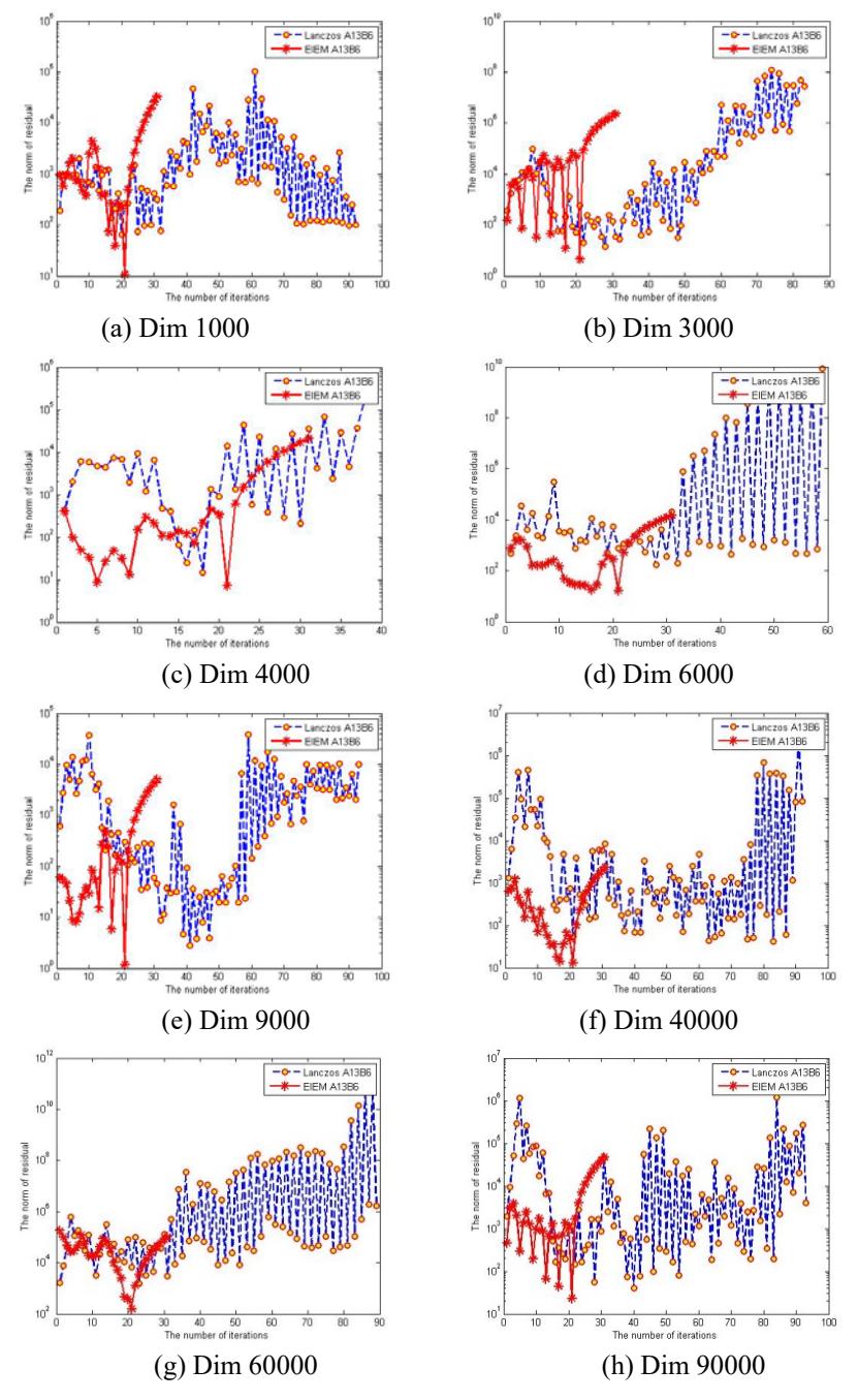
Figure 4 Performance of Lanczos A13/B6 and EIEM A13/B6 on a variety of SLEs. Blue and red curves illustrate the residual norms of respectively Lanczos A13/B6 and EIEM A13/B6.
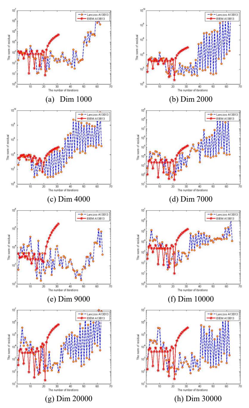
Figure 5 Performance of Lanczos A13/B13 and EIEM A13/B13 on a variety of SLEs. Blue and red curves illustrate the residual norms of respectively Lanczos A13/B13 and EIEM A13/B13 .
5.2 Discussion
Overall, the approximate solutions generated by the new algorithms, EIEM A13/B6 and EIEM A13/B13, were better than those from all of the previous iterates generated by the Lanczos-type algorithms alone. The residual norms of the iterates generated by both algorithms were smaller than all residual norms of the iterates generated by algorithms A13/B6 and A13/B13 individually. This is clearly visible in Tables 1 and 2. This was even worse for Lanczos A13/B13, where breakdown occurred in every SLE. There were, however, some cases where the new method seemed unsuccessful. It occurred, for instance, on the SLEs of dimensions 30000, 60000 and 70000 for algorithm EIEM A13/B6, and on the SLE of dimension 9000 for algorithm EIEM A13/B13.
Our above observations are supported by Figures 5 and 6. As can be seen in both figures, the residual norms of the iterates generated by either A13/B6 or A13/B13 individually, became larger and larger so that convergence was never reached. In contrast, both EIEM A13/B6 and EIEM A13/B13 generated approximate solutions with small residual norms, even smaller than the smallest residual norm of the iterates generated by A13/B6 and A13/B13 alone. Note that the residual norms of the solutions generated by EIEM A13/B6 and A13/B13 are still larger than the ambitious tolerance of 1E-13 we have imposed. One way of improving accuracy is perhaps to restart the algorithms with the final iterates, which are rather good. A discussion of the restarting strategy can be found in [31].
6 Summary
We have introduced a new approach to solving high-dimension SLEs by embedding an interpolation model in Lanczos-type algorithms, called EIEMLA. We implemented this approach for algorithms A13/B6 and A13/B13, which are new Lanczos-type algorithms. Experimentally, the idea enables us to find a good solution in terms of the residual norm, i.e. the solutions must have smaller residual norms than all of the previous iterates generated by algorithms A13/B6 and A13/B13. This helps avoid breakdown in both algorithms since we interpolate over a low number of iterations. Further investigation is required to find a prediction strategy, such as a regression, that fits the data in such a way that the embedded model produces better iterates still.
Acknowledgements
The experiments using formulas A13/B6 and A13/B13 were carried out by a coworker with one of my students, therefore my thanks go to Alifhar Juliansyah.