
1 Introduction
A landslide is the displacement of slope material, such as rock, soil and debris or a mixture of such materials, down a slope [1,2]. According to Bachri and Sheresta [3], landslide disasters in Indonesia are affected by the tropical climate conditions, with high rainfall occurring annually [4]. Such disasters cause damage and disruption and are a threat to the human population [5], where casualties and property losses can be considerable. They can also do damage to industry and the environment [6,7]. Landslides can be the result of modifications to nature by human activities [8], and contribute significantly to the evolution of landforms [9]. The size of potential damage depends on the nature of the landslide itself [10].
Investigation of landslides applying various methods of assessment has been receiving increased attention in recent years. There are several methods to study the problem of landslides, such as geophysical methods to identify the sliding plane, methods for predicting geotechnical slope stability, geo-information methods (satellite imagery and overlay) for landslide susceptibility interpretation, geochemical methods to identify clay content, and so on. Recent researches have used geoelectric methods to investigate this problem because they are not subjective. The interpretation and analysis of resistivity values depends on local geological conditions, which can be confirmed by drilling for soil samples (coring) [11] as well as with methods based on geo-information. Meanwhile, geotechnical and geochemical methods are objective because they are based on the physical properties of the landslide material discovered by testing samples in the laboratory or by modeling.
One indication of a potential landslide area is the formation of a sliding plane on the slope with soil/rock material on top of it. Landslide debris that slides down a slope with high velocity is a remarkable geological phenomenon [12]. Velocity is the most important parameter for determining the destructive potential of a landslide; only a few meters per second of landslide velocity can cause significant damage [13]. Velocity and landslide area have been proposed using landslide data from the literature [14], using a numerical simulation model [15], spatial analysis [16,17], remote sensing [18], modeling in a tank [19], and so on. Models for the estimation of landslide travel onto a horizontal surface below the slope based on the slope's geometry were then produced from the application of a simple energy conservation formula. The estimate uncertainty of travel distance and velocity of landslides should be considered in most landslide situations and one needs to allow for this when planning in landslide-prone areas. Nevertheless, the estimate of travel distances and velocity of landslide is valuable for landslide risk assessment purposes. The estimate of potential landslide volume can be applied to predict the size of a landslide given the soil thickness or potential failure plane and to estimate the landslide hazard due to earthquakes and faults.
Landslide material in the study area is moving towards the toe of the slope, threatening to cover a highway and move down to the coastline. The movement is influenced by mechanical and hydraulic resistance factors that also affect the velocity and lateral extent of the slide. Until recently, relatively little research had been done on landslide kinematics. In an effort to understand the kinematics of landslides and to provide guidance in planning mitigation strategies, velocity estimation and geomorphological analysis are critical. In this paper, a research on the movement of landslides is reported, which used an energy conservation formula in lumped mass models to determine the estimated velocity and width range, while the estimated volume was assessed based on resistivity inversion data from the Amahusu landslide, a rotational landslide.
2 Materials and Methods
2.1 Study Area
Slope geometry and geoelectric surveys were carried out in the Amahusu hills, Nusaniwe subdistrict, Ambon, Indonesia, geographically located at coordinates 03043'59.37"-03043'55.57" southern latitude, and 128008'23.12"-128008'19.30" eastern longitude (Figure 1) [20]. On June 30, 2013, a landslide occurred in Amahusu. The landslide geometry was about 250.50 m long and about 2-5 m thick. The average width of the landslide was 60 m, with the largest width of 85 m located at the center. The area of the landslide was about 4,783 m2 . The elevations of the crown of the landslide and the landslide legs were respectively 142 m.asl and 14 m.asl, with a steep slope of 84.2%. The rock in the Amahusu landslide contained Ambon volcanic rock, sandy clay and soil debris.
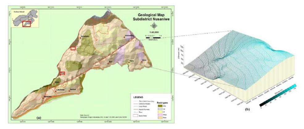
Figure 1 (a) Geological map of Nusaniwe subdistrict, (b) topographical profile of Amahusu landslide.
2.2 Estimation of Landslide Volume with Geoelectric Method
One indication of a potential landslide area is the formation of a sliding plane on a slope. A sliding plane is caused by differences between a layer and the overburden layer underneath [21]. The sliding plane can be detected using geoelectrical resistivity because there is a high resistivity contrast between the top soil layers and the impermeable bottom layers. Direct-current electrical survey is used to determine the subsurface resistivity distribution by measuring the electrical potential difference between a pair of potential electrodes on the ground surface with a current applied through a pair of current electrodes. Resistivity is measured as apparent resistivity [22] following Eq. (1):
\[\rho_a = K \frac{\Delta V}{I} \tag{1}\] with \(\rho a\) is the apparent resistivity \((\Omega.m)\), \(\Delta V\) is the potential difference (volts), I is the current strength (A), \(K = \pi n(n+1)a\) is the geometry factor (m) for the Wenner-Schlumberger configuration [23], a is the distance between the electrodes (m), and n = 1, 2, 3, 4...
Determining the volume of a landslide is a more difficult task, which requires information on the surface and sub-surface geometry of the failure slope. The physical basis for this observation is poorly understood, but its implications are enormous. Such a trend means that landslides are intrinsically scale independent, i.e. they retain a geometrical similarity independent of the scale at which they occur. For a homogeneous slope, the only length scale of the problem is the slope size upon which the slide occurs [24]. In the absence of any other length scale, simple scaling predicts that the landslide's thickness should correlate with its lateral dimensions and both should correlate with the steepness of the slope.
A 2D cross-section arc model representing a landslide can be transformed into a cone ball representing the landslide in 3D so that the length of the surface of the landslide is the diameter of the cap and the thickness of the landslide. Thus, using the landslide's surface length scale (which in 3D would be the diameter of the cap) and the landslide's thickness it is easy to calculate the volume of the correlating 3D landslide cap. Based on the 2D resistivity cross-section there is a resistivity contrast between the layers on the sliding plane. The sliding plane can be divided into two planes, A and B (marked by a black dotted line in the model). The region underneath the sliding plane is in the area of geoelectric measurement. Based on these measurements, the maximum depth of the sliding plane above A and B is obtained. Based on geological mapping, the width and length of the sliding plane are obtained so that the volumes of A and B can be determined. The method of calculating the volume of soil above a sliding plane uses the formula for a half-ellipse.
2.3 Model Estimate of Travel Distance and Velocity
In places with height differences, soil located at higher elevations tends to move downwards due to propulsive forces. In addition to the force that drives down the mass there are also resisting forces on the sliding plane that work against the ground movement so that the position of the soil remains stable. A propulsive force such as gravity can cause a landslide.
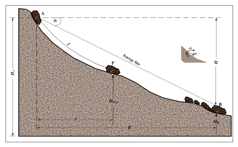
Figure 2 Slope geometry of lumped mass model (modified from [25]).
Figure 2 shows a slope geometry, where point A, the starting position of the soil mass containing potential energy (Ep), starts to move along the slope and the potential energy is transformed into kinetic energy (Ek). During movement a certain amount of energy is lost due to friction (Er). Thus, at any given location defined by height \(H_P(x)\) and distance x, the following law of conservation of energy applies:
\[mgH_A = mgH_P(x) + \int_{x_A}^{x} \mu gm \cos \beta(x) d\ell + \frac{1}{2} mv^2\] (2)
From Eq. (2) we can infer that the estimated velocity of landslide v(x) can be calculated according to topography \(H_P(x)\) as follows:
\[v(x) = \sqrt{2g} \sqrt{\left(H_A - H_P(x)\right) - \mu(x - x_A)}\] (3)
where \(H_A - H_P(x) = H\) is the elevation difference at the landslide site, \(\mu(x-xA)\) is the height of the energy line, \(\mu = H / R\) is the friction coefficient, and R is the travel distance of the landslide (m).
3 Results and Discussion
3.1 Estimated Landslide Volume using Geoelectric Survey
This result is based on a recent investigation of the Amahusu landslide in the hills of Kayu Besi Nusaniwe, Ambon. This event occurred on July 29, 2013. The landslide type was clearly rotational. A geoelectric survey was carried out using a resistivity method with Wenner-Schlumberger configuration and the topography was obtained by GPS survey. Geoelectric lines of the track were not taken parallel to the slope due to the very steep and narrow topography, so that the measurements needed to be supplemented with slope values to complete the overall data. The parameters were then adjusted to determine the resistivity values of the field.
The values of rock resistivity (,m) resulting from analysis and interpretation using standard resistivity, observation of the rocks in the field, and other secondary data were arranged for the survey area. Interpretation of the details of the calculation and data processing, in principle for each datum point on the resistivity section, shows that the resistivity values were between 5 and 500 m (Figure 3) with the following details: the first resistivity group (I), with a low resistivity value (< 30 m), was interpreted to be soil, clay and clay powder, and was generally brown to reddish brown in color. This material was generally loose/weathered, and porous enough to pass water through at a low rate. The water content makes this material more conductive. The second resistivity group (II), with medium resistivity values (30-60 m), was interpreted to be sand, sandy clay with fine to coarse grain, clay and gravel. These rocks were found at various depths and thicknesses. This material is generally loose/weathered and porous enough to pass water through at a high rate. The third resistivity group (III), with a high resistivity value (> 60 m), was interpreted to be sandy loam with fine to moderate grain, and compact claystone. These rocks were found at various depths and thicknesses. This material is generally compact and acts as bedrock in almost the entire survey area.
Analysis of the resistivity and subsurface interpretation (Figure 6) indicated that the study area is a landslide prone area, since it is estimated that there is slip between the soil bedding layer and the compact and hard rocks, i.e. there is contrast between high, medium and low resistivity layers. The landslide potential of the slide area lies in the medium resistivity group with sand or clay sand overlying a high resistivity group in the form of compact claystone. The slip field in this path can be triggered by high rainfall with a long duration before and during the landslide. This causes the rainwater to permeate the porous rock (claystone and compact stone), so there is a possibility that the water will accumulate in the layer and the layer easily decays, thus increasing the rock/soil mass as well as increasing the load on the slope and making the slope instable. The rainwater also permeates the impermeable layer of rock that is suspected to be sandy clay (medium resistivity group). The existence of weathered rock or undecayed bedrock and moisture content above the clay causes the layer of rock to become slippery, so that rocks on top of it slide down the slope. Thus, the sandy clay acts as a sliding plane, which can cause a landslide. The sliding plane of a landslide can be determined by observing a crease in the soil on the track where the subsurface is visible. It can also be seen from the difference in solidity of the soil structure in places where the landslide occurred and in places where it did not occur. The potential slide plane in the study area is approximately indicated by the dotted lines in vertical crosssections AMH-01 to AMH-06 (Figure 3). The landslide movement is classified as a rotational slide.
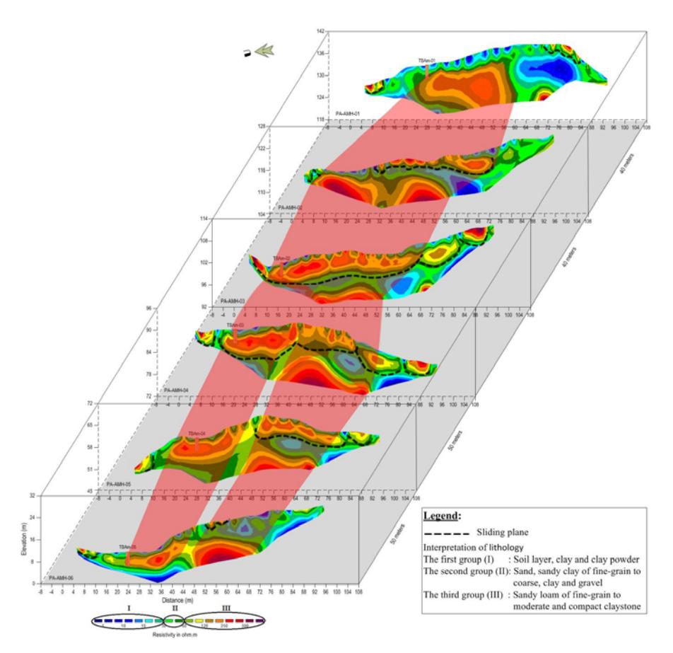
Figure 3 Stacked section of true resistivity at line AMH-01-06 [26].
Sectional image modeling of resistivity values was conducted by measuring resistivity points on six lines with a spacing of 4 m and a path length of 100 m in the north-south direction and with a distance between each line of 40 m. The topography of these lines is at elevations of 10.5-139.0 m above sea level (m.asl). The parameters were obtained in the form of apparent resistivity values. These values were correlated to obtain a picture of the physical conditions of the rock below the surface through interpretation of the inversion using an anomaly map in the form of a stacked cross-section of true resistivity (Figure 6). The interpretation results indicated that the sliding plane lies at a depth of 2-5 m, which can be interpreted as clay sand with resistivity values of 30 Ωm, as shown in Figure 6. The identification process was done on six lines, which were dominated by values of low to high resistivity with AMH-01 as the apparent resistivity distribution, which is different from the AMH_02-03 profile possibly occurring at a depth of more than 5 m. Meanwhile, at the same depth, the apparent resistivity distribution of AMH-04 resembles that of AMH-02-03. The sliding zone was estimated to lie at the position x = 8-58 m, as can be seen from the AMH-02 profile, and was expected to occur in the AMH-03 profile at the position x = 25-55 m up to a position of about x = 25 m in the AMH-01 profile. There is also a possible sliding zone below a depth of d = 5 m at position x = 25-52 m in the AMH-04-06 profile. The sliding plane is obtained from the resistivity contrast between two neighboring rock layers. Generally, at the beginning of the track in the study area there is some exposure of overburden that has a relatively higher resistivity than the other zones that allegedly contain a large amount of clay rock, which results in a decline of the resistivity value of the medium.
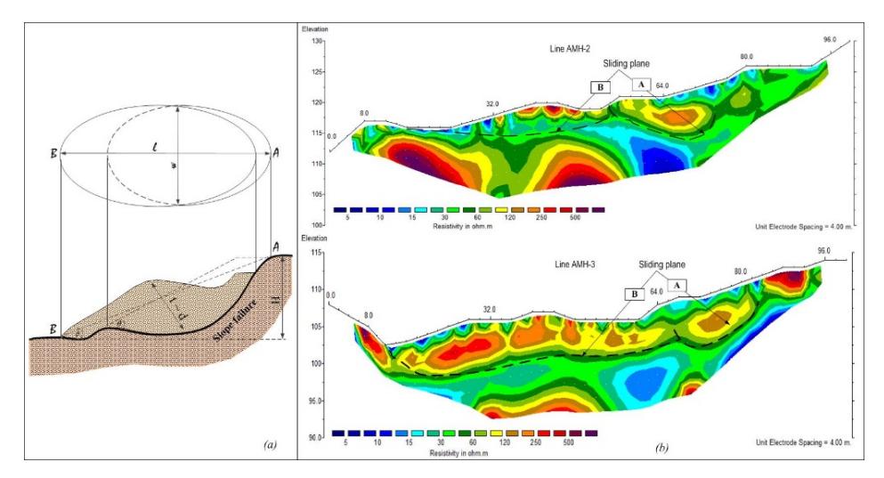
Figure 4 Sliding plane estimated from the resistivity profile at cross-sections AMH-2 and AMH-3 and the corresponding volume configuration.
This estimate was obtained by combining the position of the upper sliding plane (A) and the lower sliding plane (B) on the 2D resistivity cross-section map for each path with resistivity values of about 30 m (Figure 4). Figure 4 shows the measuring lines at each research location. Thus, by inserting sliding plane variables for each line, a prediction of the landslide volume is obtained. The result of this calculation is shown in Figure 5. The diagram of the estimated landslide volume (Figure 5) indicates different types of landslides due to different locations being triggered by different mechanisms. This shows that the ratio between the thickness of the landslide and the length of the landslide surface is extremely sensitive to the mechanical properties of the soil, where the soil strength reduces with decreasing depth from the ground surface. The estimated landslide volume of the current landslide is 70,954 m3 , while the estimated volume of a potential landslide in the down position sliding plane A and B is 50,603 m3 .
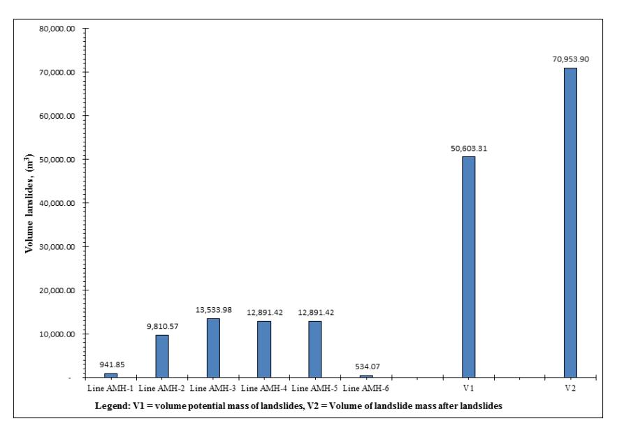
Figure 5 Estimation results for volume of Amahusu landslide.
There is a difference between the estimated landslide volume and the estimated mass potential volume of the landslide because the estimated landslide volume is determined from information on the surface and sub-surface geometry of the failure slope. Meanwhile, the estimated value of the potential volume of the landslide mass is determined based on the contrast in resistivity between one layer in the sliding plane and the layer above it. The distribution of the landslide volume can be applied to estimate the expected size of a landslide, considering the thickness of the soil or the potential failure of the slope, so that the resulting avalanche danger can be estimated.
If the landslide mass is on a steep slope, a re-occurrence of a landslide at the same location is possible. This is because the layer has a heavier load and incoming water cannot penetrate the layer of clay so that the water will be accumulated on top of the bottom layer, resulting in saturation of the landslide mass, followed by drastic reduction of soil strength, which in turn reduces its safety against sliding. This anomalous alteration will occur if the disturbances on the slope and the chance to shift to the south or the north. On the other hand, in the horizontal direction, the landslide distribution is in the direction of the sliding plane, headed to the western-sea cliff toward houses and the coastline.
3.2 Estimate of Travel Distance and Velocity of Landslide
After the volume of the landslide mass was estimated, the travel distance and velocity of the landslide were calculated based on slope geometry data obtained in previous studies [25,26] (Figures 4 and 6(a)), where the mass of unstable soil moves on the sliding plane from southeast-northwest toward the bottom of the slope and local roads to the coastline. The calculation step began with making a downhill track based on the measurement and slope parameter data. These data were used to estimate the travel distance and velocity of the landslide based on the previous equation. Field observation of the elevation along the trajectory of the Amahusu landslide allows estimation of velocity between two points along the track. First, the coefficient of friction of runout for the first part of the trajectory, xA=0, was estimated using Eq. (3) simplified to \(v_1(x) = \sqrt{2g} \sqrt{(\tan \beta - \mu)x}\):
\[v_1(x) = \begin{cases} 1.119\sqrt{x} & \text{for } \beta = 27.15^0 \\ 1.611\sqrt{x} & \text{for } \beta = 30.17^0 \\ 2.453\sqrt{x} & \text{for } \beta = 37.07^0 \end{cases}\] (with \(\mu = 0.45\))
For the second part of the trajectory, when the center of mass has moved to the position of \(x_A = 69.00\) m, the velocity estimate is:
\[v_2(x) = \sqrt{600.543 - 1.985x} \tag{5}\]
The results of the analysis Eq. 4 and Eq. 5 as a function of distance (x) are presented in Figures 6(b) and 6(c). The equations were used to obtain an estimate of the maximum velocity of the landslide based on the maximum height obtained from the curve as shown in Table 1.
This shows that after the rock/soil mass starts to move from the crest of the sliding plane and slides with great velocity along the slope, the velocity will reduce with increasing travel distance. Vertical drop \(H_{\rm max}\) refers to the height from the elevation of the occurred landslide to the elevation of the landslide
accumulation and reflects the total energy of the landslide movement with landslide volume.
| Table 1 | Results of parametric study of Amahusu Landslide. |
|---|
| Parameters | Value | Units |
|---|---|---|
| Height difference, H | 136.00 | m.asl |
| Angle of friction, | 24.18 | 0 |
| Coefficient of friction, | 0.45 | |
| Runout distance, R | 302.91 | m |
| For slope angles, = 27o | ||
| Maximum velocity, v(x)max | 15.27 | m/s |
| Distance, x | 185.00 | m |
| Maximum height, H(x)max | 101.00 | m.asl |
| For slope angles, = 30o | ||
| Maximum velocity, v(x)max | 18.45 | m/s |
| Distance, x | 131.00 | m |
| Maximum height, H(x)max | 82.20 | m.asl |
| For slope angles, = 37o | ||
| Maximum velocity, v(x)max | 21.25 | m/s |
| Distance, x | 75.00 | m |
| Maximum height, H(x)max | 62.71 | m.asl |
Generally, the greater the vertical drop, the greater the potential energy, the greater the landslide sliding speed, the farther the runout distance, and the greater the hazard region. The mass movement of a rotational type landslide was found in the Amahusu landslide, not that of a translational type landslide. For the velocity of a rotation type landslide, the result of the analysis is 15.27- 21.25 m/s for slope angle (27-30°). Translational landslides have lower velocity than rotational landslides. Landslide velocity depends on material properties, motion mechanism and the characteristics of the path. Some lithologies are expected to produce extremely rapid movement: quick clays, loess, loose spoil tips, etc.
The analysis (Figure 6) showed that travel distance gets smaller with increasing landslide velocity at different slope angles for a soil mass friction angle of 24°. Thus, the estimated maximum landslide velocity is 18.45 m/s at 131.00 m from the main scarp and is located at the maximum height of 82.20 m.asl with gradients reaching 30°. For a slope of 37°, the estimated maximum landslide velocity is 21.25 m/s at 75.00 m and is located at a maximum height of 62.71 m.asl. The greater the ratio between the slope angle and the soil mass friction angle, the higher the landslide velocity and the lower the energy line. Conversely, the smaller the slope angle relative to the soil mass friction angle, the lower the landslide velocity and the higher the energy line.
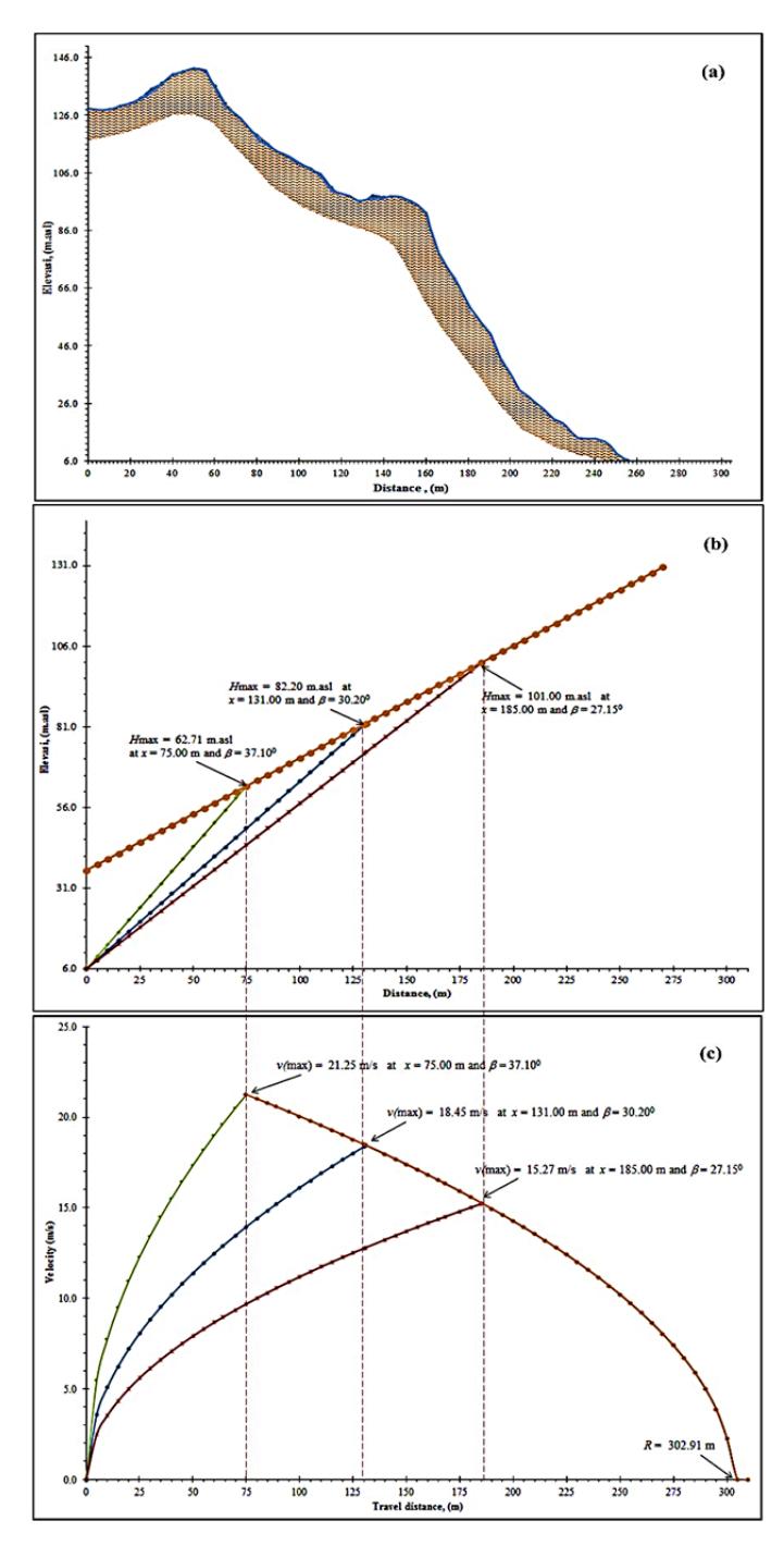
Figure 6 (a) Amahusu landslide profile slice, (b) estimated maximum height, (c) estimated velocity of the Amahusu landslide.
Derivatives of landslide velocity against position x are infinite at the beginning and at the end, which means that significant changes of landslide velocity occur at these positions. According to this simple physics analysis the landslide stops abruptly. Thus, the estimation of the landslide velocity gain depends only on the shape of the landslide path, because the trajectory of the available energy content is controlled by the frictional model. From the analysis, the velocity of the sliding mass is initially very high and gradually reduces until it reaches the downstream slope. It possessed great kinetic energy, which could destroy homes and alter geomorphology. Landslide velocity changes greatly depend on the altitude of the slope and the deposition of landslide material.
The results of the landslide velocity prediction analysis can provide an overview of the landslide imprint. The estimated maximum velocity in the Amahusu landslide was different from that for landslides at other sites. This difference depends on the height, distance runout, slope, pseudo-friction angle and local geological stratigraphy. The landslide speed is lower if there is water contained in the slope, whereas if water does not play a role (slope in a dry state), then the speed of the landslide is higher. Thus, water greatly reduces the velocity and range of a landslide with the same geometry and coefficient of friction. High velocity of the moving mass is present in rotation type landslides, in general exceeding 15 m/s. Our velocity prediction of the Amahusu landslideapproaches the results reported by Helm [25] and Iverson [27]. Individual landslides indicate that the derivative of velocity to distance is not limited to the starting and end points of the track, which means that the velocity changes very rapidly around these points of passage. Thus, according to the analysis of this simple energy line, the landslide stops abruptly (transit time) and further pushes the landslide material in front of it down the slope. This means, that the steepness of the slope is not sufficient to overcome a major obstacle, applying a relatively smaller retaining force over a longer distance. The larger the angle of the slope, the faster the landslide mass releases the total enormous energy so that the distance traveled by the landslide material until it settles at the foot of the slope is greater, despite the loss of energy. Loss of energy occurs at some cracking points, whereas along the energy line it is assumed to be linear because the mass of the landslide is considered to be constant. If the water factor plays a role, the speed will decrease. Very high landslide velocity values are found in cracked areas and carry large energies that decrease along slopes with a long range. Alteration of landslide velocity follows an energy line that involves gradual material changes during movement.
4 Conclusion
Estimation of volume movement of the Amahusu landslide with the application of a simple energy conservation formula and resistivity inversion was successfully carried out. The results of the analysis provided an estimated landslide volume of about 70,954 m³ and an estimated potential landslide volume of about 50,603 m³. The differences between both values are because the landslide volume estimation requires information on the surface and subsurface geometry of the failure slope, while the potential landslide volume estimation is base on the geometry of the sliding plane. The landslide mass moved over a distance of 302.91 m with an estimated maximum velocity of 21.25 m/s at about 75.00 m from the onset of the landslide, and reached a maximum height of 62.71 m.asl at a slope angle of 37°. As expected, fluctuations in the landslide parameters of velocity, travel distance and volume were influenced by the angle of the slope.
The accuracy of the landslide volume estimate depends on the measurement of the geometry of the failure slope. The constraints can be overcome by borehole inclinometers at many different locations while digital image analysis and digital terrain models based on a geographical information system can be combined to obtain optimum results.
Acknowledgements
The authors would like to express their thanks to the Earth Physics Laboratory, Faculty of Mathematics and Natural Sciences, Unpatti Ambon, and the Department ESDM of Maluku province for their assistance in completing the data retrieval.