1 Introduction

The survival of the plant population is under great threat in places where excessive quantities of toxic metals and contaminants are released into the environment by industries, agriculture and acid rain. Industries produce heavy metals and radioactive substances. Fertilizers, pesticides and insecticides used in agricultural fields for production enhancement contain toxic metals, which can cause harm to the plant population. Thornley [1] studied plant physiology entirely using mathematical modeling but Lacointe [2] pointed out the narrow scope of the models Thornley proposed. The failure to represent topological and geometrical differences in Lacointe's models was brought to light by Godin, et al. [3]. A mathematical model consisting of the combined effects of toxic metals and soil chemistry for the study of the adverse effect of toxic metals on the biomass of trees was proposed by Leo, et al. [4]. The model developed by Leo was further modified and applied to other plants by Guala, et al. [5,6]. A twocompartment mathematical model proposed by Misra and Kalra [7,8] was used to study the adverse effect of toxicity on individual plant growth by showing the overall decrease in uptake and concentration of nutrients and plant biomass in the root and shoot compartments. The nature of the roots of transcendental and exponential polynomials can be studied using Rouche's theorem [9]. Ruan and Wei [10,12] studied the nature and distribution of the roots of exponential polynomials for the study of stability with time lag using Rouche's theorem; the phenomenon of population dynamics was represented using non-linear delay differential equations. Population dynamics stability was studied by Kubiaczyk and Saker [11]. The reduction of plant biomass under the effect of toxicants with time lag was studied by Naresh, et al. [13]. Shukla, et al. [14] studied how crop yield is adversely affected by environmentally degraded soil. The dynamics of a multiteam prey-predator system under the effect of time lag was studied by Sikarwar and Misra [15]. Naresh, et al. [16] studied how excessive industrial waste results in toxic uptake by plants and how the intermediate toxic products formed affect the intrinsic growth rate of plant biomass and carrying capacity. The global stability of population growth with the help of non-linear delay differential equations was studied by Huang, et al. [17]. Zhang, et al. [18] developed a neural network model and discussed the nature of the roots of a 5thdegree exponential polynomial.

Although a great deal of work has been done on plant growth under the effect of toxicants, the use of delay differential equations is rare in this field. In the presence of toxic metals in the soil, the nutrient uptake by plants and the nutrient transfer from the root compartment to the shoot compartment gets delayed. The nutrient use efficiency is adversely affected too, which leads to a decrease in structural dry weight. Hence, this time delay due to toxic metals in the soil is directly responsible for a decrease in the structural dry weight of the plant, which is a measure of delayed and reduced plant growth. Considering the above fact, a two-compartment mathematical model is proposed in this paper for the study of individual plant growth. A delay parameter is introduced in the term containing the utilization coefficient. Also, the complex behavior giving rise to Hopf bifurcation was studied.

2 Mathematical Model

2.1 Assumptions of the Model

We made the following assumptions in the mathematical model:

• 1. Nutrient uptake by the roots is hindered by the presence of toxic metals.
• 2. There is less transfer of nutrients from the root compartment to the shoot compartment due to the presence of toxic metals in the soil.

• 3. The nutrient concentration decreases in the root compartment as well as in the shoot compartment, resulting in a decrease of the structural dry weight of the roots and shoots respectively.
• 4. Nutrient use efficiency is affected by the presence of toxic metals, resulting in a decrease of the structural dry weight of the shoots.

2.2 Model Formulation

Let \(N_1\) and \(W_1\) represent the nutrient concentration and the structural dry weight of the root compartment respectively. Let \(N_2\) and \(W_2\) represent the nutrient concentration and the structural dry weight of the shoot compartment respectively. Let \(H_s\) be the concentration of heavy metals in the soil. These notations lead to the following model, a system of the following non-linear delay differential equations:

\[\frac{dN_1}{dt} = (U_n - \alpha H_s) - \frac{T}{R_n} N_1 - \mu W_1 N_1 (t - \tau) - d_1 N_1 \tag{1}\]

\[\frac{dN_2}{dt} = \frac{T(H_S)}{R_n} N_1 - \mu W_2 N_2 - d_2 N_2 \tag{2}\]

\[\frac{dW_1}{dt} = r_1(N_1, H_S)W_1 - \Delta_1 W_1^2\] (3)

\[\frac{dW_2}{dt} = r_2(N_2, H_S)W_2 - \Delta_2 W_2^2 \tag{4}\]

\[\frac{dH_S}{dt} = I - \alpha_1 H_S N_1 - \Delta H_S \tag{5}\] with initial conditions:

\(N_1(0) > 0, N_2(0) > 0, W_1(0) > 0, W_2(0) > 0, H_s(0) > 0\) for all \(t \ge 0\) and \(N_1(t - \tau) = \varepsilon\), constant for all \(t \in [0, \tau]\).

Here, \(r_1(N_1, H_S)\) and \(r_2(N_2, H_S)\) have the following forms:

\[r_{1}(N_{1}, H_{s}) = \frac{\rho N_{1}}{1 + \gamma_{1} H_{s}} - \beta_{1}(H_{s}), \quad \frac{\partial r_{1}(N_{1}, H_{s})}{\partial H_{s}} < 0, \frac{\partial r_{1}(N_{1}, H_{s})}{\partial N_{1}} > 0 \text{ for } N_{1} > 0, H_{s} > 0\] \[r_{2}(N_{2}, H_{s}) = \frac{\rho N_{2}}{1 + \gamma_{2} H_{s}} - \beta_{2}(H_{s}), \quad \frac{\partial r_{2}(N_{2}, H_{s})}{\partial H_{s}} < 0, \frac{\partial r_{2}(N_{2}, H_{s})}{\partial N_{2}} > 0 \text{ for } N_{2} > 0, H_{s} > 0\] \[T(H_{s}) = \frac{T}{1 + T_{0} H_{s}}, \quad \beta_{1}(H_{s}) = \beta_{10} + \beta_{11} H_{s}, \quad \beta_{2}(H_{s}) = \beta_{20} + \beta_{21} H_{s}.\]

The system parameters are defined as follows:

\(r_2(N_2, H_S)\) and \(r_1(N_1, H_S)\) are the growth rates of the shoots and roots under the effect of heavy metals \(H_S\), respectively; they are dependent on the availability of nutrients. T is the nutrient transfer rate from the root compartment to the shoot

compartment. \(R_n\) is the resistance to the transportation of nutrients. \(T(H_s)\) is the nutrient transfer rate from the root compartment to the shoot compartment, which is hampered by the presence of heavy metals \(H_s\). \(R_n\) is the aversion to transportation of the nutrients. \((U_n - \alpha H_s)\) is the uptake rate by the plant, which is inhibited due to the presence of heavy metals in the soil. \(\mu\) is the consumption coefficient, or utilization coefficient. \(\rho\) is the effeciency of nutrient utilization. \(\beta_{10}\) is the natural decay of \(W_1\). \(\beta_{20}\) is the natural decay of \(W_2\). \(d_1\) is the natural decay of \(N_1\). \(d_2\) is the natural decay of \(N_2\). \(\Delta_2\) and \(\Delta_1\) are self-limiting growth rates \(W_2\) and \(W_1\), respectively. \(\beta_{11}\) and \(\beta_{21}\) are the damage rates of \(W_1\) and \(W_2\)due to \(H_s\), respectively. I is the input rate of the toxic metals. \(\Delta\) is the first-order decay rate of \(H_s\). \(\alpha_1\) is the depletion rate of \(H_s\) due to the reaction between \(H_s\)and \(N_1\). \(T_0\) is a stress parameter, which measures the increase in resistance to nutrient transport from the root compartment to the shoot compartment due to the presence of toxic metals in the soil. \(\gamma_1\) and \(\gamma_2\) are parameters measuring the decrease in nutrient use efficiency due to the presence of toxic metals in the plant. All parameters, \(\alpha, I, \rho, \Delta, \mu, U_n, \alpha_1, T_0, \gamma_1, \gamma_2, \Delta_1, \Delta_2\), were taken to be positive constants.

3 Analysis of Model

3.1 Boundedness

The boundedness of the solutions of the model given by Eqs. (1)-(5) is given by Lemma 3.1.

Lemma 3.1. The model has all its solutions in the region \(D_1 = \left\{ (N_1, N_2, W_1, W_2, H_s) \in R_+^{5} \colon 0 \leq N_1 + N_2 + \frac{\mu}{\rho} W_1 + \frac{\mu}{\rho} W_2 \leq \frac{U_n}{\varphi}, H_{sl} \leq H_s \leq H_{su} \right\},\) as \(t \to \infty\) for all positive initial values \(\{N_1(0), N_2(0), W_1(0), W_2(0), H_s(0), N_1(t - \tau) = \varepsilon \ \forall t \in [0, \tau]\} \in D_1 \subset R_+^{5},\) where \(\varphi = \min(d_1, d_2, \beta_{10}, \beta_{20}).\)

Proof. Consider the following function: \(F(t) = N_1(t) + N_2(t) + \frac{\mu}{\rho} W_1(t) + \frac{\mu}{\rho} W_2(t)\)

\[\frac{dF(t)}{dt} = \frac{d}{dt} \left[ N_1(t) + N_2(t) + \frac{\mu}{\rho} W_1(t) + \frac{\mu}{\rho} W_2(t) \right]\]

Using Eqs. (1)-(4) and \(\varphi = \min(d_1, d_2, \beta_{10}, \beta_{20})\) and assumption \(N_1(t) \approx N_1(t-\tau)\) as \(\to \infty\), \(\Rightarrow \frac{dF(t)}{dt} \le U_n - \varphi F(t)\).

By usual comparison theorem, when \(\rightarrow \infty\): \(F(t) \leq \frac{U_n}{a}\)

\[N_1(t) + N_2(t) + \frac{\mu}{\rho} W_1(t) + \frac{\mu}{\rho} W_2(t) \le \frac{U_n}{\omega}\]

Also, \[F(t) \ge 0\]. So, \(0 \le N_1(t) + N_2(t) + \frac{\mu}{\rho} W_1(t) + \frac{\mu}{\rho} W_2(t) \le \frac{U_n}{\varphi}\).

From Eq. (5): \(\frac{dH_S}{dt} = I - \alpha_1 H_S N_1 - \Delta H_S\), \(\frac{dH_S}{dt} \le I - \Delta H_S\), then by usual comparison theorem, when \(t \to \infty\): \(H_S \le \frac{I}{\Lambda} = H_{SU}\).

Again, from Eq. (5), we get \(\frac{dH_S}{dt} = I - \alpha_1 H_S N_1 - \Delta H_S\) i.e. \(\frac{dH_S}{dt} \ge I - \alpha_1 H_S \frac{U_n}{\varphi} - \Delta H_S\)

\[\frac{dH_s}{dt} \ge I - \vartheta_3 H_s\] where \(\vartheta_3 = \left(\frac{\alpha_1 U_n}{\omega} + \Delta\right)\).

By usual comparison theorem, when \(t \to \infty\): \(H_s \ge \frac{1}{\vartheta_3} = H_{sl}\), so \(H_{sl} \le H_s \le H_{su}\). This completes the proof.

The boundedness lemma proves that since all quantities (the nutrient concentrations in the roots and shoots, the toxic metals in the soil and the structural dry weights of the roots and shoots) are real quantities, their individual values as well as their interactional combinations can never be negative and will be finite at all times.

3.2 Positivity of Solutions

For the positivity of the solutions we need to show that all solutions of the system given by Eqs. (1)-(5), where the initial conditions are \(N_1(0) > 0\), \(N_2(0) > 0\), \(W_1(0) > 0\), \(W_2(0) > 0\), \(W_1(0) > 0\), \(W_2(0) > 0\) for all t > 0 and \(V_1(t - \tau) = \varepsilon \forall\), \(t \in [0, \tau]\), the solution \((N_1(t), N_2(t), W_1(t), W_2(t), H_s(t))\) of the model stays positive \(\forall t > 0\).

From Eq. (2): \[\frac{dN_2}{dt} = \frac{T(H_S)}{R_n} N_1 - \mu W_2 N_2 - d_2 N_2, \quad \frac{dN_2}{dt} \ge -\left(\mu \frac{U_n}{\varphi} + d_2\right) N_2, \text{ i.e.}\] \[N_2 \ge c_1 e^{-\left(\mu \frac{U_n}{\varphi} + d_2\right)t}. \text{ Here, } c_1 \text{ is an integration constant, hence } N_2 > 0 \text{ as } t \to \infty.\]

The same argument holds for \(N_1\), \(W_1\), \(W_2\), \(H_S\).

Thus, all variables remain positive, which shows that the system persists.

3.3 Interior Equilibrium of the Model

The system of Eqs. (1)-(5) has one feasible positive interior equilibrium \(E_1(N_1^*, N_2^*, W_1^*, W_2^*, H_S^*)\), where

\[W^*_1 = \frac{1}{\Delta_1} \left[ \frac{\rho}{1 + \gamma_1 H^*_s} N^*_1 - (\beta_{10} + \beta_{11} H^*_s) \right] > 0,\] provided \(\rho N^*_1 > (1 + \gamma_1 H^*_s) (\beta_{10} + \beta_{11} H^*_s)\) \[W^*_2 = \frac{1}{\Delta_2} \left[ \frac{\rho}{1 + \gamma_2 H^*_s} N^*_2 - (\beta_{20} + \beta_{21} H^*_s) \right] > 0,\] provided \(\rho N^*_2 > (1 + \gamma_2 H^*_s) (\beta_{20} + \beta_{21} H^*_s)\) \[N^*_1 = \frac{I - \Delta H^*_s}{\alpha_1 H^*_s} \text{ provided } I > \Delta H^*_s,\] \[N^*_2 = \frac{-g_2 + \sqrt{g^2_2 - 4g_1 g_3}}{2g_1} > 0\] where \[g_1 = \frac{\mu \rho}{\Delta_1 (1 + \gamma_1 H^*_s)}\], \(g_2 = \left(d_1 - \frac{\mu(\beta_{10} + \beta_{11} H^*_s)}{\Delta_1}\right)\), \(g_3 - \frac{T(I - \Delta H^*_s)}{R_n \alpha_1 H^*_s (1 + T_0 H^*_s)}\)

the value of \(H_S^*\) is given by the positive root of the equation

\[\begin{split} \gamma_{2}(\alpha + \delta_{3}\Delta){H^{*}}_{s}^{4} - [\gamma_{2}(U_{n} - \delta_{1}\Delta + \delta_{3}I) - (\alpha + \delta_{3}\Delta)]{H^{*}}_{s}^{3} - \\ [U_{n} + \delta_{3}I + \delta_{1}(\Delta - I\gamma_{2}) - \delta_{2}\Delta^{2}]{H^{*}}_{s}^{2} - I(2\Delta\delta_{2} - \delta_{1}){H^{*}}_{s} + \delta_{2}I^{2} = 0 \end{split}\] where \(\delta_{1} = \frac{1}{\alpha}\Big(\frac{T}{R_{n}} + d_{1} - \frac{\mu\beta_{10}}{\Delta_{1}}\Big), \delta_{2} = \frac{\mu\rho}{\Delta_{1}\alpha_{1}^{2}}, \delta_{3} = \frac{\pi\beta_{11}}{\Delta_{1}\alpha_{1}}\)

the \(4^{th}\)-degree polynomial in \(H_s^*\) will have at most two positive roots, provided:

\[\begin{aligned} \gamma_2(U_n - \delta_1 \Delta + \delta_3 I) &> (\alpha + \delta_3 \Delta), \\ (U_n + \delta_3 I + \delta_1 \Delta) &> \delta_1 I \gamma_2 + \delta_2 \Delta^2, \\ k_1 &> 2\Delta \delta_2 \end{aligned}\]

However, due to the positivity of \(N_1^*\) only one feasible positive root will exist, provided \(I > \Delta H_s^*\).

Theorem 3.1. Let \(\zeta_1, \zeta_2, ..., \zeta_m\) all be non-negative and \(\zeta_i^j (j = 0, 1, 2, ..., m: i = 1, 2, ..., n)\) be constants. As \((\zeta_1, \zeta_2, ..., \zeta_m)\) vary, the sum of the orders of the zeros of exponential polynomial \(P(\chi, e^{-\chi \zeta_1}, ..., e^{-\chi \zeta_m})\) on the open right half plane can change only if a zero appears on or crosses the imaginary axis, where

\[P(\chi, e^{-\chi \zeta_1}, \dots, e^{-\chi \zeta_m}) = \chi^n + \zeta_1^0 \chi^{n-1} + \dots + \zeta_{n-1}^0 \chi^n + \zeta_n^0 + [\zeta_1^1 \chi^{n-1} + \dots + \zeta_{n-1}^1 \chi^n + \zeta_n^1] e^{-\chi \zeta_1} + \dots + [\zeta_1^m \chi^{n-1} + \dots + \zeta_{n-1}^m \chi^n + \zeta_n^m] e^{-\chi \zeta_m}\]

Ruan and Wei [10,12] proved this theorem using Rouche's theorem.

3.4 Stability Analysis of Interior Equilibrium Point and Local Hopf Bifurcation

The exponential characteristic equation about equilibrium \(E_1\) is given by

\[(\lambda^5 + A_1 \lambda^4 + A_2 \lambda^3 + A_3 \lambda^2 + A_4 \lambda + A_5) + (B_1 \lambda^4 + B_2 \lambda^3 + B_3 \lambda^2 + B_4 \lambda + B_5) e^{-\lambda \tau} = 0\] (6)

\(+P_1P_{12}(P_{10}(P_7+P_{25})+P_{25}P_7-P_{10}P_{22}))\)

Here,

\[\begin{split} A_1 &= -(P_1 + P_7 + P_{13} + P_{19} + P_{25}), \\ A_2 &= (P_7 P_{13} + P_{13} P_{25} + P_{25} P_7 + P_{25} P_{10} + P_{11} P_{13} + P_1 P_7 + P_1 P_{13} + P_1 P_{25} + P_7 P_{19} + P_{13} P_{19} + P_{19} P_{25}), \\ A_3 &= -\Big( (P_1 + P_{19})(P_7 P_{13} + P_{13} P_{25} + P_{25} P_7 + P_{10} P_{25}) + P_1 P_{19}(P_7 + P_{13} + P_{25}) + P_1 P_{13}(P_7 + P_{19} + P_{25}) + P_7 P_{13} P_{25} + P_{10} P_{13} P_{22} \Big), \\ A_4 &= \Big( P_1 P_{19}(P_7 P_{13} + P_{13} P_{25} + P_{25} P_7 + P_{25} P_{10}) + (P_1 + P_{19})(P_7 P_{13} P_{25} + P_{10} P_{13} P_{22}) \end{split}\]

\[A_5 = - \Big( P_1 P_{19} (P_7 P_{13} P_{25} + P_{10} P_{13} P_{22}) + P_{11} P_{13} P_{19} (P_{25} P_7 - P_{10} P_{22}) \Big),\]

\[B_{1} = \mu W_{1}^{*},\] \[B_{2} = -\mu W_{1}^{*}(P_{1} + P_{13} + P_{19} + P_{25}),\] \[B_{3} = \mu W_{1}^{*}((P_{1} + P_{19})(P_{13} + P_{25}) + P_{1}P_{19} + P_{1}P_{13} + P_{13}P_{25}),\] \[B_{4} = -\mu W_{1}^{*}(P_{1}P_{19}(P_{13} + P_{25}) + P_{13}(P_{1} + P_{19}) + P_{1}P_{13}(P_{19} + P_{25})),\]

\[B_3 = \mu W^*_1 (P_1 P_{19} P_{13} P_{25} + P_{11} P_{19} P_{13} P_{25})\] where,

\[\begin{split} P_1 &= -(\mu W^*_{\ 2} + d_2), \quad P_2 = \frac{T}{R_n(1 + T_0 H^*_s)}, \quad P_3 = -\mu N^*_{\ 2}, \quad P_4 = 0, \quad P_5 = \\ &\frac{-TT_0 N^*_{\ 1}}{R_n(1 + T_0 H^*_s)^2}, \quad P_6 = 0, P_7 = -\left(\frac{T}{R_n} + d_1\right), \quad P_8 = 0, P_9 = 0, P_{10} = -\alpha, P_{11} = \\ &\frac{\rho W^*_{\ 2}}{1 + \gamma_2 H^*_s}, P_{12} = 0, P_{13} = \frac{\rho N^*_{\ 2}}{(1 + \gamma_2 H^*_s)^2} - (\beta_{20} + \beta_{21} H^*_s) - 2\Delta_2 W^*_{\ 2}, \qquad P_{14} = 0 \;, \\ P_{15} &= -\left(\frac{\rho N^*_{\ 2} W^*_{\ 2} \gamma_2}{(1 + \gamma_2 H^*_s)^2} + \beta_{21} W^*_{\ 2}\right), \quad P_{16} &= \frac{\rho W^*_{\ 1}}{1 + \gamma_1 H^*_s}, \quad P_{17} = 0, \quad P_{18} = 0, \quad P_{19} = \\ &\frac{\rho N^*_{\ 1}}{(1 + \gamma_1 H^*_s)^2} - (\beta_{10} + \beta_{11} H^*_s) - 2\Delta_1 W^*_{\ 1}, \qquad P_{20} &= -\left(\frac{\rho N^*_{\ 1} W^*_{\ 1} \gamma_1}{(1 + \gamma_1 H^*_s)^2} + \beta_{11} W^*_{\ 1}\right), \\ P_{21} &= 0, P_{22} &= -\alpha_1 H^*_s, P_{23} = 0, P_{24} = 0, P_{25} &= -(\alpha_1 N^*_{\ 1} + \Delta). \end{split}\]

Let \(\lambda = i\omega\) be a root of Eq. (6), so:

\[((i\omega)^{5} + A_{1}(i\omega)^{4} + A_{2}(i\omega)^{3} + A_{3}(i\omega)^{2} + A_{4}(i\omega) + A_{5})\] \[+(B_{1}(i\omega)^{4} + B_{2}(i\omega)^{3} + B_{3}(i\omega)^{2} + B_{4}(i\omega) + B_{5})e^{-(i\omega)\tau} = 0\] \[(i\omega^{5} + A_{1}\omega^{4} - iA_{2}\omega^{3} - A_{3}\omega^{2} + iA_{4}\omega + A_{5})\] \[+(B_{1}\omega^{4} - iB_{2}\omega^{3} - B_{3}\omega^{2} + iB_{4}\omega + B_{5})(\cos\omega\tau - i\sin\omega\tau) = 0\]

Separating real and imaginary parts:

\[(\omega^{5} - A_{2}\omega^{3} + A_{4}\omega) + (B_{4}\omega - B_{2}\omega^{3})\cos\omega\tau - (B_{1}\omega^{4} - B_{3}\omega^{2} + B_{5})\sin\omega\tau = 0\] \[(A_{1}\omega^{4} - A_{3}\omega^{2} + A_{5}) + (B_{1}\omega^{4} - B_{3}\omega^{2} + B_{5})\cos\omega\tau + (B_{4}\omega - B_{2}\omega^{3})\sin\omega\tau = 0\] (8)

Squaring and adding Eq. (7) and Eq. (8), we get:

\[\omega^{10} + a\omega^8 + b\omega^6 + c\omega^4 + d\omega^2 + r = 0 \tag{9}\] where \[a = (A_1^2 - B_1^2 - 2A_2), b = (A_2^2 - B_2^2 - 2A_4 - 2A_1A_3 + 2B_1B_3), c = (A_3^2 - B_3^2 - 2A_2A_4 + 2B_2B_4 - 2B_1B_5), d = (A_4^2 - B_4^2 - 2A_3A_5 + 2B_3B_5), r = (A_5^2 - B_5^2)\]

Let \(\omega^2 = y\), then Eq. (9) becomes:

\[y^5 + ay^4 + by^3 + cy^2 + dy + r = 0 (10)\]

Lemma 3.1. If r < 0, then Eq. (10) has at least one positive real root.

Proof. Let \[h(y) = y^5 + ay^4 + by^3 + cy^2 + dy + r\],
Here, \(h(0) = r < 0\), \(\lim_{y \to \infty} h(y) = \infty\)
so, \(\exists y_0 \in (0, \infty)\) such that \(h(y_0) = 0\)

Proof completed.

Also \[h'(y) = 5y^4 + 4ay^3 + 3by^2 + 2cy + d\]
Let \(h'(y) = 0\)
\(5y^4 + 4ay^3 + 3by^2 + 2cy + d = 0\) (11)

which becomes \[x^4 + px^2 + qx + s = 0\] (12)

where \[= y + \frac{a}{5}\], \(p = \frac{3b}{5} - \frac{6a^2}{25}\), \(q = \frac{2c}{5} + \frac{6ab}{25} + \frac{8a^3}{125}\), \(s = \frac{d}{5} - \frac{2ac}{25} + \frac{3a^2b}{125} - \frac{3a^4}{625}\)

If q = 0, then the four roots of Eq. (12) are:

\[x_1 = \sqrt{\frac{-p + \sqrt{D}}{2}}, x_2 = -\sqrt{\frac{-p + \sqrt{D}}{2}}, x_3 = \sqrt{\frac{-p - \sqrt{D}}{2}}, x_4 = -\sqrt{\frac{-p - \sqrt{D}}{2}}\]

Thus, \(y_i = x_i - \frac{a}{5}\), i = 1,2,3,4 are the roots of Eq. (10) where \(D = p^2 - 4s\).

Lemma 3.2. Suppose \(r \ge 0\) and q = 0.

• 1. If D < 0, then Eq. (10) has no positive real roots.
• 2. If \(D \ge 0\), \(p \ge 0\), \(s \ge 0\), then Eq. (10) has no positive real roots.
• 3. If (I) and (II) are not satisfied, then Eq. (10) has positive real roots iff \(\exists\) at least one \(y^* \in (y_1, y_2, y_3, y_4)\) such that \(y^* > 0\) and \(h(y^*) \le 0\).

Proof.

• I. If D < 0, then Eq. (11) has no positive real roots. Since \(\lim_{y \to \infty} h(y) = \infty\), we have h'(y) > 0 for \(y \in R\). Hence \(h(0) = r \ge 0\) implies h(y) has no zero in \((0, \infty)\).
• II. Condition \(D \ge 0\), \(p \ge 0\), \(s \ge 0\) implies that h'(y) has no zero in \((-\infty, \infty)\). This is similar to (I), i.e. h(y) has no zero in \((0, \infty)\).
• 4. The sufficiency is obvious.

Hence, we only need to prove the necessity. If \(D \ge 0\), we know that Eq. (12) has only four roots \(x_1, x_2, x_3\) and \(x_4\), i.e. Eq. (11) has only four roots, \(y_1, y_2, y_3\) and \(y_4\), and at least \(y_1\) is a real root. Without loss of generality, we assume that \(y_1, y_2, y_3\) and \(y_4\) are all real. This implies that h(y) has at most four stationary points \(y_1, y_2, y_3\) and \(y_4\). If this is not true, then we have that either \(y_1 \le 0\) or \(y_1 > 0\) and \(\min[h(y_i): y_i > 0, i = 1,2,3,4] > 0\). If \(y_1 \le 0\), then h'(y) has no zero in \((0, \infty)\), since \(h(0) = r \ge 0\) is the strict minimum of h(y) for \(y \ge 0\), which implies h(y) > 0 in \((0, \infty)\). If \(y_1 > 0\) and \(\min[h(y_i): y_i > 0, i = 1,2,3,4] > 0\). Since h(y) is a derivable function and \(\lim_{y\to\infty} h(y) = \infty\), we have \(\min_{y>0} h(y) = \min[h(y_i): y_i > 0, i = 1,2,3,4] > 0\). The necessity is proved. This completes the proof.

Next, we assume that \(q \neq 0\). Consider the resolvent of Eq. (12):

\[q^{2} - 4(v - p)\left(\frac{v^{2}}{4} - s\right) = 0\]\ni.e. \(v^{3} - pv^{2} - 4sr + 4ps - q^{2} = 0\) (13)

By Cardan formula, Eq. (13) has the following three roots:

\[v_1 = \left(-\frac{q_1}{2} + \sqrt{D_1}\right)^{1/3} + \left(-\frac{q_1}{2} - \sqrt{D_1}\right)^{1/3} + \frac{p}{3},\] \[v_2 = \sigma \left(-\frac{q_1}{2} + \sqrt{D_1}\right)^{1/3} + \sigma^2 \left(-\frac{q_1}{2} - \sqrt{D_1}\right)^{1/3} + \frac{p}{3},\] \[v_3 = \sigma^2 \left(-\frac{q_1}{2} + \sqrt{D_1}\right)^{1/3} + \sigma \left(-\frac{q_1}{2} - \sqrt{D_1}\right)^{1/3} + \frac{p}{3},\] where \(p_1 = -\frac{p^2}{3} - 4s\), \(q_1 = -\frac{2p^3}{27} + \frac{8ps}{3} - q^2\), \(D_1 = \frac{p_1^3}{27} + \frac{q_1^2}{4}\), \(\sigma = \frac{1 + \sqrt{3}i}{2}\)

Let \(v_* = v_1 \neq p\), then Eq. (12) becomes:

\[x^{4} + v_{*}x^{2} + \frac{v_{*}^{2}}{4} - \left[ (v_{*} - p)x^{2} - qx + \frac{v_{*}^{2}}{4} - s \right] = 0\] (14)

For Eq. (14), Eq. (12) implies that the formula in square brackets is a perfect square. If \(v_* > p\), then Eq. (14) becomes:

\[\left(x^2 + \frac{v_*}{2}\right)^2 - \left(\sqrt{v_* - p}x - \frac{q}{2\sqrt{v_* - p}}\right)^2 = 0\]

After factorization, we get:

\[x^2 + \sqrt{v_* - p}x - \frac{q}{2\sqrt{v_* - p}} + \frac{v_*}{2}\] and \(x^2 - \sqrt{v_* - p}x - \frac{q}{2\sqrt{v_* - p}} + \frac{v_*}{2}\)

So, the four roots of Eq. (12) are:

\[x_1 = \frac{-\sqrt{v_* - p} + \sqrt{D_2}}{2}, x_1 = \frac{-\sqrt{v_* - p} - \sqrt{D_2}}{2}, x_3 = \frac{-\sqrt{v_* - p} + \sqrt{D_3}}{2}, x_4 = \frac{-\sqrt{v_* - p} - \sqrt{D_3}}{2}\] where \[D_2 = -v_* - p + \frac{q}{2\sqrt{v_* - p}}\] and \(D_3 = -v_* - p - \frac{q}{2\sqrt{v_* - p}}\)

Then \(y_i = x_i - \frac{a}{5}\), i = 1,2,3,4 are the roots of Eq. (10). Thus, we have the following result:

Lemma 3.3. Suppose that \(r \ge 0\), \(q_1 \ne 0\) and \(v_* > p\).

• 1. If \(D_2 < 0\) and \(D_3 < 0\), then Eq. (10) has no positive real roots.
• 2. If (I) is not satisfied, then Eq. (10) has positive real roots iff \(\exists\) at least one \(y^* \in (y_1, y_2, y_3, y_4)\) such that \(y^* > 0\) and \(h(y^*) \le\).

Proof. The proof is similar to Lemma 3.2 and we omit it. Finally, if \(v_* < p\), then Eq. (14) becomes \(\left(x^2 + \frac{v_*}{2}\right)^2 - \left(\sqrt{p - v_*}x - \frac{q}{2\sqrt{p - v_*}}\right)^2 = 0\) (15)

Let \(\bar{y} = \frac{q}{2(v-v_*)} - \frac{a}{5}\). Hence, we have the following result:

Lemma 3.4. Suppose that \(r \ge 0\), \(q_1 \ne 0\) and \(v_* < p\), then Eq. (10) has positive real roots iff \(\frac{q^2}{4(n-v_*)^2} + \frac{v_*}{2} = 0\) and \(\bar{y} > 0\) and \(h(\bar{y}) \le 0\).

Proof. Assume Eq. (14) has a real root \(x_0\) satisfying \(x_0 = \frac{q}{2(p-v_*)}\), \(x_0^2 = -\frac{v_*}{2}\), which implies that \(\frac{q^2}{4(p-v_*)^2} + \frac{v_*}{2} = 0\). Therefore, Eq. (14) has a real root \(x_0\) iff \(\frac{q^2}{4(p-v_*)^2} + \frac{v_*}{2} = 0\). The rest of the proof is similar to Lemma 3.2 and we omit it.

Suppose Eq. (10) possesses positive roots. In general, we suppose that it has 5 positive roots denoted by \(y^*_{i}\), i = 1,2,3,4,5. Then Eq. (9) has 5 positive roots \(\omega_i = \sqrt{y^*_{i}}\), i = 1,2,3,4,5.

We have: \[\cos \omega \tau = \frac{A_6}{(B_4 \omega - B_2 \omega^3)^2 + (B_1 \omega^4 - B_3 \omega^2 + B_5)^2}\] which gives \[\tau = \frac{1}{\omega} \left[ \cos^{-1} \left( \frac{A_6}{(B_4 \omega - B_2 \omega^3)^2 + (B_1 \omega^4 - B_3 \omega^2 + B_5)^2} \right) + 2j\pi \right], \quad j = 0,1,2,3,...\] where \[A_6 = -\left( (B_1\omega^4 - B_3\omega^2 + B_5)(A_1\omega^4 - A_3\omega^2 + A_5) + (B_4\omega - B_2\omega^3)(\omega^5 - A_2\omega^3 + A_4\omega) \right)\]

Let \[\tau_k^{(j)} = \frac{1}{\omega_k} \left[ \cos^{-1} \left( \frac{A_6}{(B_4 \omega - B_2 \omega^3)^2 + (B_1 \omega^4 - B_3 \omega^2 + B_5)^2} \right) + 2j\pi \right]; k = 1,2,3,4,5.; j = 0,1,2,3,....\]

Then \(\mp i\omega_k\) is a pair of purely imaginary roots of Eq. (6), where \(\tau = \tau_k^{(j)}\), k = 1,2,3,4,5.; j = 1,2,3,... we have \(\lim_{j\to\infty} \tau_k^{(j)} = \infty\), k = 1,2,3,4,5.

Thus, we can define:

\[\tau_0 = \tau_{k_0}^{(j_0)} = \min_{1 \le k \le 4, j \ge 1} \left[ \tau_k^{(j)} \right], \ \omega_0 = \omega_{k_0}, \ y_0 = y_{k_0}^*\] (16)

Lemma 3.5. Suppose that \(u_1 > 0\), \((u_1u_2 - u_3) > 0\), \(u_3(u_1u_2 - u_3) + u_1(u_5 - u_1u_4) > 0\), \((u_2u_5 + u_3u_3)(u_1u_2 - u_3) + u_1u_4(u_5 - u_1u_4) > 0\), \(u_5 > 0\).

Where \[u_1 = (A_1 + B_1), u_2 = (A_2 + B_2), u_3 = (A_3 + B_3), u_4 = (A_4 + B_4), u_5 = (A_5 + B_5).\]

• 1. If any one of the following condition holds:
  • (i) r < 0,
  • (ii) \(r \ge 0, q = 0, D \ge 0\) and p < 0 and \(s \le 0\) and there exists a \(y^* \in (y_1, y_2, y_3, y_4)\) such that \(y^* > 0\) and \(h(y^*) \le 0\),

• (iii) \(r \ge 0, q \ne 0, v_* > p, D_2 \ge 0 \text{ or } D_3 \ge 0\) and there exists a \(y^* \in (y_1, y_2, y_3, y_4)\) such that \(y^* > 0\) and \(h(y^*) \le 0\)
• 2. \(r \ge 0, q \ne 0, v_* < p, \frac{q^2}{4(p-v_*)^2} + \frac{v_*}{2} = 0, \overline{y} > 0\) and \(h(\overline{y}) \le 0\), then a negative real part will exist in all roots of Eq. (6) when \(\tau \in [0, \tau_0)\).
• 3. If any one of the Conditions (i)-(iv) of (I) are not satisfied, then negative real parts will exist in all roots of Eq. (6) for all \(\tau \ge 0\).

Proof. When \(\tau = 0\), Eq. (6) becomes:

\[\lambda^{5} + (A_{1} + B_{1})\lambda^{4} + (A_{2} + B_{2})\lambda^{3} + (A_{3} + B_{3})\lambda^{2} + (A_{4} + B_{4})\lambda\]\[+ (A_{5} + B_{5}) = 0\]\[\lambda^{5} + u_{1}\lambda^{4} + u_{2}\lambda^{3} + u_{3}\lambda^{2} + u_{4}\lambda + u_{5} = 0\](17)

All roots of Eq. (17) have negative real parts iff the supposition of Lemma 3.5 holds (Routh-Hurwitz's criteria).

From Lemmas 3.1-3.4., we know that if Conditions (i)-(iv) of (I) are not satisfied, then none of the roots of Eq. (6) will have zero real parts for all \(\tau \ge 0\).

If one of the Conditions (i)-(iv) holds, when \(\tau \neq \tau_k^{(j)}\), k = 1,2,3,4,5; \(j \geq 1\), then none of the roots of Eq. (6) will have zero real parts and \(\tau_0\) is the minimum value of \(\tau\) for which the roots of Eq. (6) are purely imaginary. This lemma is concluded by using Theorem 3.1.

Let

\[\lambda(\tau) = \psi(\tau) + i\omega(\tau) \tag{18}\] be the roots of Eq. (6) satisfying: \(\psi(\tau_0) = 0\), \(\omega(\tau_0) = \omega_0\). Then we have the following lemma:

Lemma 3.6. Suppose \(h'(y_0) \neq 0\). If \(\tau = \tau_0\), then \(\mp i\omega_0\) is a pair of simple purely imaginary roots of Eq. (6). Moreover, if the conditions of Lemma 3.5 (I) are satisfied, then \(\frac{d}{d\tau}(Re\lambda(\tau_0)) > 0\).

Proof. Substituting \(\lambda(\tau)\) into Eq. (6) and differentiating both sides with respect to \(\tau\) we get:

\[\left(\frac{d\lambda}{d\tau}\right)^{-1} = \frac{\left(5\lambda^4 + 4A_1\lambda^3 + 3A_2\lambda^2 + 2A_3\lambda + A_4\right)e^{\lambda\tau} + \left(4B_1\lambda^3 + 3B_2\lambda^2 + 2B_3\lambda + B_4\right)}{(B_1\lambda^4 + B_2\lambda^3 + B_3\lambda^2 + B_4\lambda + B_5)} - \frac{\tau}{\lambda}\]

By calculation, we have:

\[\left[ (5\lambda^4 + 4A_1\lambda^3 + 3A_2\lambda^2 + 2A_3\lambda + A_4)e^{\lambda\tau} \right]_{\tau=\tau_0} =\]

\[A_7 \cos \omega_0 \tau + A_8 \sin \omega_0 \tau + i(-A_8 \cos \omega_0 \tau + A_7 \sin \omega_0 \tau)\] \[(4B_1 \lambda^3 + 3B_2 \lambda^2 + 2B_3 \lambda + B_4)_{\tau = \tau_0} = B_4 - 3B_2 \omega_0^2 + i\omega_0 (2B_3 - 4B_1 \omega_0^2)\] \[(B_1 \lambda^4 + B_2 \lambda^3 + B_3 \lambda^2 + B_4 \lambda + B_5)_{\tau = \tau_0} =\] \[\omega_0^2 (B_2 \omega_0^2 - B_5) + i\omega_0 (B_5 - B_3 \omega_0^2 + B_1 \omega_0^4)\] where \(A_7 = (5\omega_0^4 - 3A_3 \omega_0^2 + A_4)\), \(A_8 = (4A_1 \omega_0^3 - 2A_3 \omega_0)\)

Then we have:

\[\left(\frac{d\operatorname{Re}\lambda(\tau_0)}{d\tau}\right)^{-1} = \frac{y_0 h'(y_0)}{A_9} \tag{19}\] where \[A_9 = \omega_0^2 [(B_2 \omega_0^3 - B_5 \omega_0)^2 + (B_5 - B_3 \omega_0^2 + B_1 \omega_0^4)^2]\]

Thus we have sign:

\[\left[\frac{d \operatorname{Re}\lambda(\tau_0)}{d\tau}\right] = \operatorname{sign}\left[\left(\frac{d \operatorname{Re}\lambda(\tau_0)}{d\tau}\right)^{-1}\right] = \operatorname{sign}\left[\frac{y_0 h'(y_0)}{A_9}\right]\](20)

Notice that \(A_9\), \(y_0 > 0\).

Thus, applying the Lemmas 3.1-3.6, we have the following theorem:

Theorem 3.2. Let \(\omega_0\), \(y_0\), \(\tau_0\) and \(\lambda(\tau)\) be defined by Eqs. (16) to (18), respectively. Assuming that the supposition of Lemma 3.5 holds,

• 1. If the Conditions (i)-(iv) of Lemma 3.5 are not satisfied, then all roots of Eq. (6) have negative real parts for all \(\tau \ge 0\).
• 2. If one of the Conditions (i)-(iv) of Lemma 3.5 is satisfied, then all roots of Eq. (6) have negative real parts when \(\tau \in [0, \tau_0)\); when \(\tau = \tau_0\) and \(h'(y_0) \neq 0\), then \(\mp i\omega_0\) is a pair of purely imaginary roots of Eq. (6) and all other roots have negative real parts. In addition, \(\frac{d \operatorname{Re}\lambda(\tau_0)}{d\tau} > 0\) and Eq. (6) has at least one root with a positive real part when \(\tau \in (\tau_0, \tau_1)\), where \(\tau_1\) is the first value of \(\tau > \tau_0\) such that Eq. (6) has purely imaginary roots.

3.5 Numerical Method

A numerical method was used to find the solution of the system of delay differential equations given by Eqs. (1)-(5), considering the following parameter values: \(U_n = 10\), T = 1.5, \(R_n = 1\), \(\mu = 1.05\), \(d_1 = 0.9\), \(d_2 = 0.9\), \(\rho = 0.3\), \(\beta_{10} = 0.2\), \(\beta_{20} = 0.2\), \(\Delta_1 = 0.1\), \(\Delta_2 = 0.1\), I = 0.1, I = 0.1, I = 0.1, I = 0.1, I = 0.1, I = 0.1, I = 0.1, I = 0.1, I = 0.1, I = 0.1, I = 0.1, I = 0.1, I = 0.1, I = 0.1, I = 0.1, I = 0.1, I = 0.1, I = 0.1, I = 0.1, I = 0.1, I = 0.1, I = 0.1, I = 0.1, I = 0.1, I = 0.1, I = 0.1, I = 0.1, I = 0.1, I = 0.1, I = 0.1, I = 0.1, I = 0.1, I = 0.1, I = 0.1, I = 0.1, I = 0.1, I = 0.1, I = 0.1, I = 0.1, I = 0.1, I = 0.1, I = 0.1, I = 0.1, I = 0.1, I = 0.1, I = 0.1, I = 0.1, I = 0.1, I = 0.1, I = 0.1, I = 0.1, I = 0.1, I = 0.1, I = 0.1, I = 0.1, I = 0.1, I = 0.1, I = 0.1, I = 0.1, I = 0.1, I = 0.1, I = 0.1, I = 0.1, I = 0.1, I = 0.1, I = 0.1, I = 0.1, I = 0.1, I = 0.1, I = 0.1, I = 0.1, I = 0.1, I = 0.1, I = 0.1, I = 0.1, I = 0.1, I = 0.1, I = 0.1, I = 0.1, I = 0.1, I = 0.1, I = 0.1, I = 0.1, I = 0.1, I = 0.1, I = 0.1, I = 0.1, I = 0.1, I = 0.1, I = 0.1, I = 0.1, I = 0.1, I = 0.1, I = 0.1, I = 0.1, I = 0.1, I = 0.1, I = 0.1, I = 0.1, I = 0.1, I = 0.1, I = 0.1, I = 0.1, I = 0.1, I = 0.1, I = 0.1, I = 0.1, I = 0.1, I = 0.1, I = 0.1, I = 0.1, I = 0.1, I = 0.1, I = 0.1, I = 0.1, I = 0.1, I = 0.1, I = 0.1, I = 0.1, I = 0.1, I = 0.1, I = 0.1, I = 0.1, I = 0.1, I = 0.1, I = 0.1, I = 0.1, I = 0.1, I = 0.1, I = 0.1, I = 0.1, I = 0.1, I = 0.1, I = 0.1, I = 0.1, I = 0.1, I = 0.1, I = 0.1, I = 0.1, I = 0.1, I = 0.1, I = 0.1, I = 0.1, I = 0.1, I = 0.1, I = 0.1, I = 0.1, I = 0.1, I = 0.1, I = 0.1, I = 0.1, I = 0.1, I = 0.1, I = 0.1, I = 0.1, I = 0.1, I = 0.1, I = 0.1, I =

For the given parametric values, we have: \(E_1: N^*_1 = 1.6830, N^*_2 = 1.1057, W^*_1 = 3.0490, W^*_2 = 1.3172, H^*_S = 0.7161\). In fact, without toxic effect, \(N^*_1 = 1.7357, N^*_2 = 1.1186, W^*_1 = 3.2041, W^*_2 = 1.3574\).

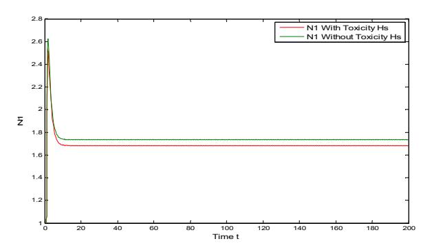
Figure 1 Graph of nutrient concentration of root \(N_1\) and time t against toxicity and without toxicity.

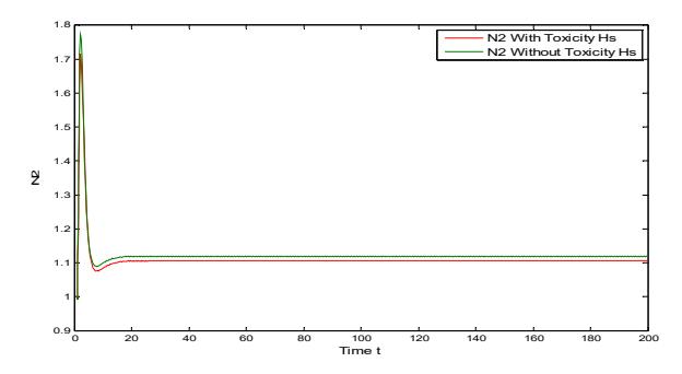
Figure 2 Graph of nutrient concentration of shoot \(N_2\) against time t with toxicity and without toxicity.

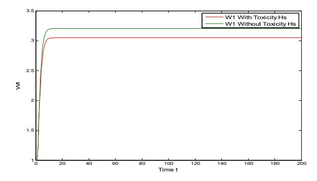
Figure 3 Graph of structural dry weight of root \(W_1\) against time t with toxicity and without toxicity.

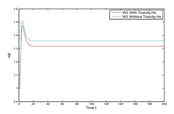
Figure 4 Graph of structural dry weight of shoot ଶ against time t with toxicity and without toxicity.

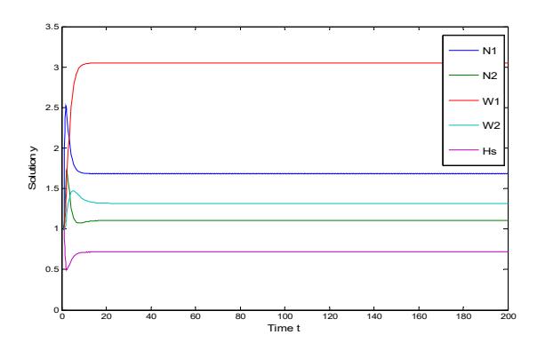
Figure 5 The interior equilibrium point E1 (1.6830, 1.1057, 3.0490, 1.3172, 0.7161) of the system is stable when there is no delay, i.e. ൌ 0.

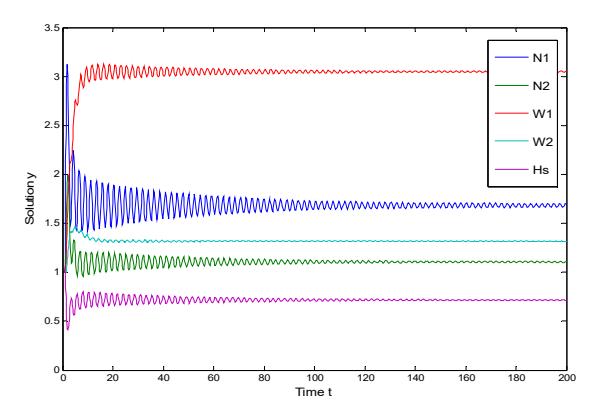
Figure 6 The interior equilibrium point E1 (1.6830, 1.1057, 3.0490, 1.3172, 0.7161) of the system is asymptotically stable with delay ൏ 0.89.

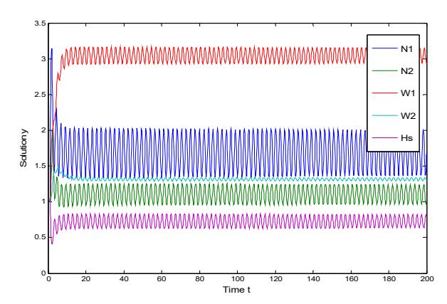
Figure 7 The interior equilibrium point E1 (1.6830, 1.1057, 3.0490, 1.3172, 0.7161) loses its stability and Hopf bifurcation occurred with delay 0.89.

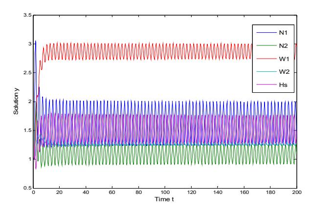
Figure 8 Increase in intake rate of toxic metal from ൌ2 to ൌ4 increases the critical value of the delay parameter from ൌ 0.89 to ൌ 0.96.

4 Sensitivity Analysis of State Variables with respect to Model Parameters

A sensitivity analysis helps to know the dependence of the system solution on perturbation in the model parameters. It tells how changes in value of parameters other than the key parameter time delay affect the stability behavior of the state variables. Two model parameters, namely nutrient transfer rate from the roots to shoot and consumption coefficient of delayed nutrients were perturbed and the corresponding numerical solution of the state variablesnutrient concentration, structural dry weights and concentration of toxic metals

ሺଵ, ଶ, ଵ, ଶ, ௦ሻ are presented graphically. The main observations are discussed in detail in Section 5 (Discussion and Conclusion).

5 Discussion and Conclusion

In this paper, we found that the equilibrium levels of the nutrient concentration in the root compartment (^{∗ ଵ} ൌ 1.7357ሻ and the shoot compartment (^{∗ ଶ} ൌ 1.1186ሻ are higher without toxic effect than the equilibrium levels of the nutrient concentration in the root compartment ሺ^{∗ ଵ} ൌ 1.6830) and the shoot compartment (^{∗ ଶ} ൌ 1.1057ሻ with toxic effect, as shown in Figures 1 and 2. We also found that the equilibrium levels of the structural dry weight of the root compartment (^{∗ ଵ} ൌ 3.2041ሻ and the shoot compartment (^{∗ ଶ} ൌ 1.3574ሻ are higher without toxic effect than the equilibrium levels of the structural dry weight of the root compartment ሺ^{∗ ଵ} ൌ 3.0490) and the shoot compartment (^{∗ ଶ} ൌ 1.3172ሻ with toxic effect, as shown in Figures 3 and 4. This shows that involvement of toxic metals decreases the nutrient concentration level and the structural dry weight of the plant.

We also studied the stability and Hopf bifurcation about the interior equilibrium of the system governed by Eqs. (1)-(5). It was concluded that when there is no time delay, interior equilibrium ଵሺ1.6830, 1.1057, 3.0490, 1.3172, 0.7161ሻ is stable, as shown in Figure 5 and as proved by Lemma 3.5 using Routh-Hurwitz's criteria. But under the same set of parameter values, we found a critical value of the parameter delay ( ൏ 0.89) below which the system is asymptotically stable, as shown in Figure 6, and unstable above that critical value, as shown in Figure 7 and as proved by Lemmas 3.1-3.4. While passing through the critical value ൌ 0.89, the system showed oscillations, hence Hopf bifurcation occurred. Furthermore, with an increase in the intake rate of toxic metal, there was more decrease in the nutrient concentration and the structural dry weight of the root and shoot compartments. The same combined adverse effect of increased intake rate of toxic metal and increased time delay is shown in Figure 8.

The sensitivity of the model solutions was established by taking different values of the parameters appearing in the system. This improves the understanding of the role played by specific model parameters.

The sensitivity analysis revealed that with an increase in the transfer rate of nutrient from the roots to the shoots, the state variables-nutrient concentration the in the root compartment and the shoot compartment, the structural dry weights of the root compartment and the shoot compartment and the concentration of toxic metals in the soil ሺଵ, ଶ, ଵ, ଶ, ௦ሻ tends towards

stability for the same set of remaining parameters, including time delay ൌ 0.89. At T = 1.5, all the abovementioned state variables show unstable behavior via Hopf bifurcation. But as the value of T is increased to T = 1.6, all the state variables start showing asymptotic stability and finally for T = 1.7, all the state variables start converging to a stable equilibrium point, as shown in Figures 9 to13.

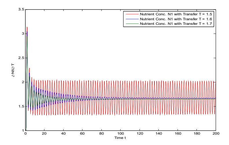
Figure 9 Time series graph of partial changes in nutrient concentration ଵ in the root compartment against different values of nutrient transfer rate .

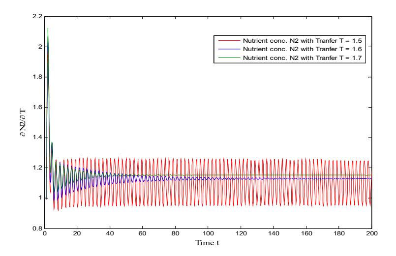
Figure 10 Time series graph of partial changes in nutrient concentration ଶ in the shoot compartment against different values of nutrient transfer rate .

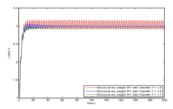
Figure 11 Time series graph of partial changes in structural dry weight ଵ of the root compartment against different values of nutrient transfer rate .

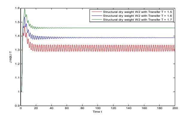
Figure 12 Time series graph of partial changes in structural dry weight ଶ of the shoot compartment against different values of nutrient transfer rate .

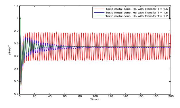
Figure 13 Time series graph of partial changes in the concentration of toxic metal ௦ in the soil against different values of nutrient transfer rate .

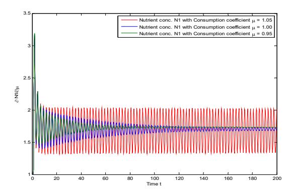
Figure 14 Time series graph of partial changes in nutrient concentration ଵ in the root compartment against different values of consumption coefficient of delayed nutrients.

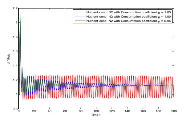
Figure 15 Time series graph of partial changes in nutrient concentration ଶ in the shoot compartment against different values of consumption coefficient .

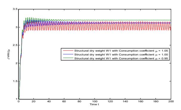
Figure 16 Time series graph of partial changes in structural dry weight ଵ of the root compartment against different values of consumption coefficient .

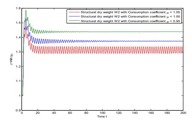
Figure 17 Time series graph of partial changes in structural dry weight ଶ of shoot compartment against different values of consumption coefficient .

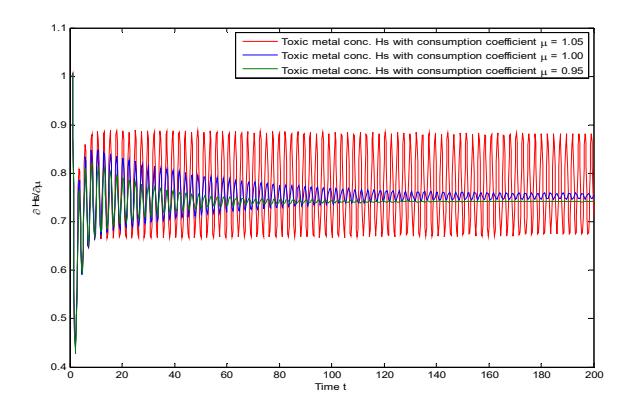
Figure 18 Time series graph of partial changes in the concentration of toxic metals ௦ in the soil against different values of consumption coefficient .

Apart from converging to stability, the structural dry weight ଶ of the shoot compartment also shows an increase when we increase the value of T from 1.5 to 1.7, as shown in Figure 12. Similarly, when we decrease the value of consumption coefficient from ൌ 1.05 to ൌ 0.95, all the abovementioned state variables start converging to a stable equilibrium, as shown in Figures 14 to Figure 18. In addition to convergence to stability, the structural dry weights ଵ and ଶ of the root and shoot compartments show an increase when we decrease the value of consumption coefficient of delayed nutrients, as shown in Figures 16 and 17.