
1 Introduction
In recent years, three-dimensional (3-D) modeling of magnetotelluric (MT) data has become more common [1,2]. It is the basis for inversion, which usually requires an initial model followed by iterative refinement. Early attempts to calculate the response of 3-D bodies used an integral equation method [3,4]. An integral equation is efficient for simple model geometries, since it is computationally fast and requires little computer storage. However, this approach is not efficient for arbitrarily complex geometries, since computer storage and computation time increase along with the complexity of the model. Alternatively, finite-difference [5-8] and finite-element [9,10] methods are commonly used. As computer power and storage increase, the application of finite-difference and finite-element methods for arbitrarily complex geometries is becoming more common.
Finite-difference methods involve approximating the Maxwell equations using either first-order or second-order equations. Finite-element methods, on the other hand, consist of numerical minimization of the energy function that corresponds to the governing differential equation under a given boundary condition (e.g. in [11]). The advantage of using a finite-element method is that one can incorporate irregular geometries to model surface topography and complex media (e.g. in [12,13]). Unfortunately, the finite-element approach, which uses nodal elements in its basis function, creates difficulties in the numerical modeling of electromagnetic field problems. This is due to possible jumps of normal components across discontinuities of material properties [14]. This difficulty can be overcome by using another type of finite-element method, which uses vector basis or vector elements that assign degrees of freedom to the edges rather than to the nodes of the elements [15,16].
In the context of MT, the application of a vector finite element method to calculate the response of 3-D bodies was introduced in [12,13,17,18]. The application of edge and nodal elements to approximate the T and Ω fields for the derived differential equation using T-Ω Helmholtz decomposition was adopted in [17]. Meanwhile, a vector finite element method to approximate the second-order Helmholtz equation of the electric field was used in [18]. Both finite-element applications in [17] and [18] discretize the modeling domain into a number of rectilinear mesh or brick elements. In contrast, the application of finite elements in [12] employs hexahedral elements (distorted bricks) to accommodate surface topography. Recently, tetrahedral elements with the addition of a goal-oriented adaptive mesh refinement approach were used in [13].
However, rather than using an iterative method (e.g. in [12] and [18]), a direct method was used here to solve the linear systems arising from the discretization process. In this research work, we aimed to provide an additional study that develops the application of vector FE modeling to geophysical electromagnetics with 3-D MT modeling examples.
2 Methods
The aim of modeling MT fields in a 3-D structural environment is to seek a solution for the vector Helmholtz equation. Similar to [18], we used vector finite elements with rectilinear mesh or brick elements to discretize the modeling domain. The vector finite elements approximate the solution of the vector Helmholtz equation that governs the physical behavior of the electromagnetic field. The electric field formulation used follows [19], so the vector Helmholtz equation can be written as:
\[\nabla \times \nabla \times \mathbf{E} - i\omega \mu_0 \sigma \mathbf{E} = 0 \tag{1}\] where E is the electric field, \(\mu_0\) is the magnetic permeability of free space, \(\omega\) is the angular frequency, and \(\sigma\) is the material conductivity. Eq. (1) together with the boundary condition at the top, bottom and sides of the modeling domain is a typical boundary-value problem, which mathematically can be written as [20]:
\[L\phi = f \tag{2}\]
In relation to Eq. (1), \(L = \nabla \times \nabla \times -i\omega \mu_0 \sigma\) is a differential operator, f = 0 implies no source term, and \(\phi = \mathbf{E}\) is an unknown quantity. Based on the Ritz method, a variational method [20], the boundary-value problem can be expressed in terms of a functional. The minimum of the functional corresponds to the governing differential equation under the given boundary condition. The approximate solution is then obtained by minimizing the functional with respect to its unknown variables.
3 Vector Finite Elements
For a numerical discretization using vector finite elements, we subdivide volume V into rectangular bricks or a rectilinear mesh. We can write the electric vector field for each element as an expansion function as follows:
\[\mathbf{E}^e = \sum_{i=1}^{12} \mathbf{N}_i^e E_i^e \tag{3}\] where \(N_i^e\) denotes the 12 vector interpolation functions, which is given by:
\[\mathbf{N}_{i\in[1-4]}^{e} = N_{xi}^{e}\hat{\mathbf{x}}, \ \mathbf{N}_{i\in[5-8]}^{e} = N_{yi}^{e}\hat{\mathbf{y}}, \ \mathbf{N}_{i\in[9-12]}^{e} = N_{zi}^{e}\hat{\mathbf{z}}\] (4)
with respect to unit vectors \(\hat{\mathbf{x}}\), \(\hat{\mathbf{y}}\) and \(\hat{\mathbf{z}}\) parallel to the x-, y-, and z-axis, respectively.
Using the local coordinate system as depicted in Figure 1, the coordinate transformation of each element can be derived by assigning a constant tangential field component to each edge of the elements. Hence, the coordinate transformations are given by \(\xi = 2\left(x - x_c^e\right)/l_x^e\), \(\eta = 2\left(y - y_c^e\right)/l_y^e\) and
\(\zeta = 2(z - z_c^e)/l_z^e\), where \(x_c^e\), \(y_c^e\), and \(z_c^e\) denote the center coordinates of the eth element. Meanwhile, \(l_x^e\), \(l_y^e\), and \(l_z^e\) denote the side lengths of the e-th element in the x-, y-, and z-directions, respectively.
Figure 1 Rectangular brick elements with local coordinate system.
The values of \(N_{xi}^e\), \(N_{vi}^e\), and \(N_{zi}^e\) in Eq. (4) can then be expressed by:
\[N_{xi}^{e} = \frac{1}{4} (1 + \eta \eta_{i}) (1 + \zeta \zeta_{i})\] (5)
\[N_{yi}^{e} = \frac{1}{4} (1 + \zeta \zeta_{i}) (1 + \xi \xi_{i})\] (6)
\[N_{zi}^{e} = \frac{1}{4} \left( 1 + \xi \xi_{i} \right) \left( 1 + \zeta \zeta_{i} \right) \tag{7}\] where \((\eta_i, \zeta_i, \xi_i)\) is the position of the midpoint on the i-th edge. Using Eq. (5)-(7), the vector interpolation functions defined in Eq. (5) have zero divergence and nonzero curl. These properties are important because they enable the problem of normal components jumping across discontinuities to be satisfied naturally. Moreover, the expansion given by Eq. (3) guarantees not only the tangential continuity across the edges but also the tangential continuity across the surface of the elements [20].
4 Variational Formulation using the Ritz Method
The variational problem, which is mathematically equivalent to the solution of Eqs. (2) or (1), may be written as:
\[\begin{pmatrix} \delta F(\mathbf{E}) = 0 \\ \text{E is defined on the boundary} \end{pmatrix} \tag{8}\]
In this case, the functional F(E) represents the total energy density function of the electric field, which can be written as [11]:
\[F(\mathbf{E}) = \frac{1}{2} \iiint_{V} \mathbf{E}^{*} \cdot (\nabla \times \nabla \times \mathbf{E} - i\omega \mu_{0} \sigma \mathbf{E}) dV\] (9)
By applying the first vector of Green's theorem, the mathematical expression of \(F(\mathbf{E})\) in Eq. (9) can be written as:
\[F(\mathbf{E}) = \frac{1}{2} \iiint_{V} \left[ \left( \nabla \times \mathbf{E}^{*} \right) \bullet \left( \nabla \times \mathbf{E} \right) - i\omega \mu_{0} \sigma \mathbf{E}^{*} \bullet \mathbf{E} \right] dV\]\[- \bigoplus_{S} \left( \mathbf{E}^{*} \times \nabla \times \mathbf{E} \right) \bullet \hat{\mathbf{n}} dS\](10)
By substituting Eq. (3) into Eq. (10), we obtain that the first term, i.e. the volume integration part, which is not zero since it only involves first-order derivatives of interpolation functions. On the other hand, the second term on the right-hand side (surface integral) can be ignored since the contributions of the surface integrals from neighboring elements will cancel each other out [18].
The assembly process of finite elements consists of substituting the expansion function in Eq. (3) into functional Eq. (10). By summing over all elements, we can write the functional in vector notation as:
\[F = \frac{1}{2} \sum_{e=1}^{M} \left( \left\{ E^{e} \right\}^{T} \left[ A^{e} \right] \left\{ E^{e} \right\} - i\omega \mu_{o} \left\{ E^{e} \right\}^{T} \left[ B^{e} \right] \left\{ E^{e} \right\} \right)\] \[(11)\] where
\[[A^e] = \iiint_{V^e} \{ \nabla \times \mathbf{N}^e \} \cdot \{ \nabla \times \mathbf{N}^e \}^T dV\] (12)
and
\[\left[B^{e}\right] = \iiint_{V^{e}} \sigma^{e} \left\{\mathbf{N}^{e}\right\} \cdot \left\{\mathbf{N}^{e}\right\}^{T} dV \tag{13}\]
M is the total number of elements and Ve denotes the volume of each element. Using Eqs. (5), (6) and (7), the integral equation in Eqs. (12) and (13) is evaluated analytically and computed numerically for every element to generate elemental matrices. Upon carrying out the summation over all elemental matrices, Eq. (11) can be written as:
\[F = \frac{1}{2} \{ E \}^{T} [A] \{ E \} - i\omega \mu_{o} \{ E \}^{T} [B] \{ E \}\] (14)
A system of algebraic linear equations is then obtained by applying the Ritz method, which amounts to taking the partial derivative of F with respect to each unknown edge field and setting it to zero. The inhomogeneous Dirichlet boundary condition is specified as the tangential component of the electric field.
It is set equal to the magnetotelluric electric field for a homogeneous or horizontally layered half-space on the boundary of the solution domain. After the boundary condition is set, the resulting equation that is given by Eq. (14) can be solved for ሼሽ. The solution of system of linear Eq. (15) can be sought using an iterative or a direct method. It is noted that Eq. (15) is well posed only if 0 i 0 [21]. In MT, a low frequency is used, so the system of linear equations arising from the discretization of Eq. (1) is ill conditioned. To overcome the problem of an ill-conditioned system, preconditioning is often employed to seek the solution of Eq. (15) when using an iterative method. However, finding a good matrix preconditioner is computationally more expensive than using a direct method [22]. For this reason we sought the solution of Eq. (15) using a direct method by employing robust direct solver PARDISO [23].
The modeling codes that we developed consist of reading the input mesh, calculating the elemental matrices, assembling the elemental matrices to produce a global matrix, imposing boundary values on the boundary vectors, and finally solving the system of algebraic linear equations. The programming language used was FORTRAN90.
\[[A]{E}-i\omega\mu_o[B]{E} = {b}\] \[\tag{15}\]
5 Results and Discussions
To test the solution of our modeling approach, the Dublin Test Model 1 (DTM1) was used for validation. The DTM1 model is designed as a reference to compare various forward codes and to know how they deal with strong resistivity contrast [24]. The resulting model responses were also compared to those of other forward calculations. The DTM1 model, shown in Figure 2, consists of three different blocks embedded in a homogeneous 100 Ω.m halfspace. The information details of the DTM1 model are summarized in Table 1.
Table 1 Dimension and Resistivity Values of the Three Blocks in DTM1.
| x (km) | y (km) | z (km) | resistivity (Ω.m) | |
|---|---|---|---|---|
| body 1 (blue) | -20 to 20 | -2.5 to 2.5 | 5 to 20 | 10 |
| body 2 (red) | -15 to 0 | -2.5 to 22.5 | 20 to 25 | 1 |
| body 3 (green) | 0 to 15 | -22.5 to 2.5 | 20 to 50 | 10000 |
Due to machine use limitations in running the modeling program on an Apple Macbook Air (1.6 GHz Intel Core i5 2 GB memory), the largest mesh size we adopted was 40 × 40 × 21 (plus 5 air layers). As depicted in Figure 3, our mesh view had equal grid spacing in the area of interest, where three blocks are located. Grid spacing was relaxed by a factor of 3 as the distance increases outside the area of interest. Using this grid-spacing configuration, our models extended to 2000 km in the x- and y-directions. Here, we compare our response along with other responses using different forward codes and different mesh sizes (shown in Table 2). Comparison of the response curve was computed for a range of frequencies at a particular point of interest, located at the center site (x = y = 0 km), as denoted by circle in Figure 3(a). The dataset for comparison was obtained from [25].
Table 1 Comparison Method of Forward Calculation and Number of Cells/Elements of DTM1.
| Code | User | Mesh (number of cells) |
|---|---|---|
| FD [5] | Randall Mackie | 92×95×73 (without air layers) |
| FD [19] | Marion Miensopust | 39×40×18 (1-2.5 km) (plus 7 air layers) |
| FE [12] | Nuree Han & Tae Jong Lee | 48×47×31 |
| FE (this work) | Rudy Prihantoro | 40x40×21 (plus 5 air layers) |
FD = finite difference, FE = finite element.
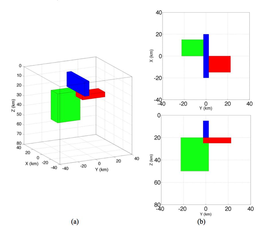
Figure 2 DTM1: (a) three-dimensional view, (b) plan view, (c) section view.
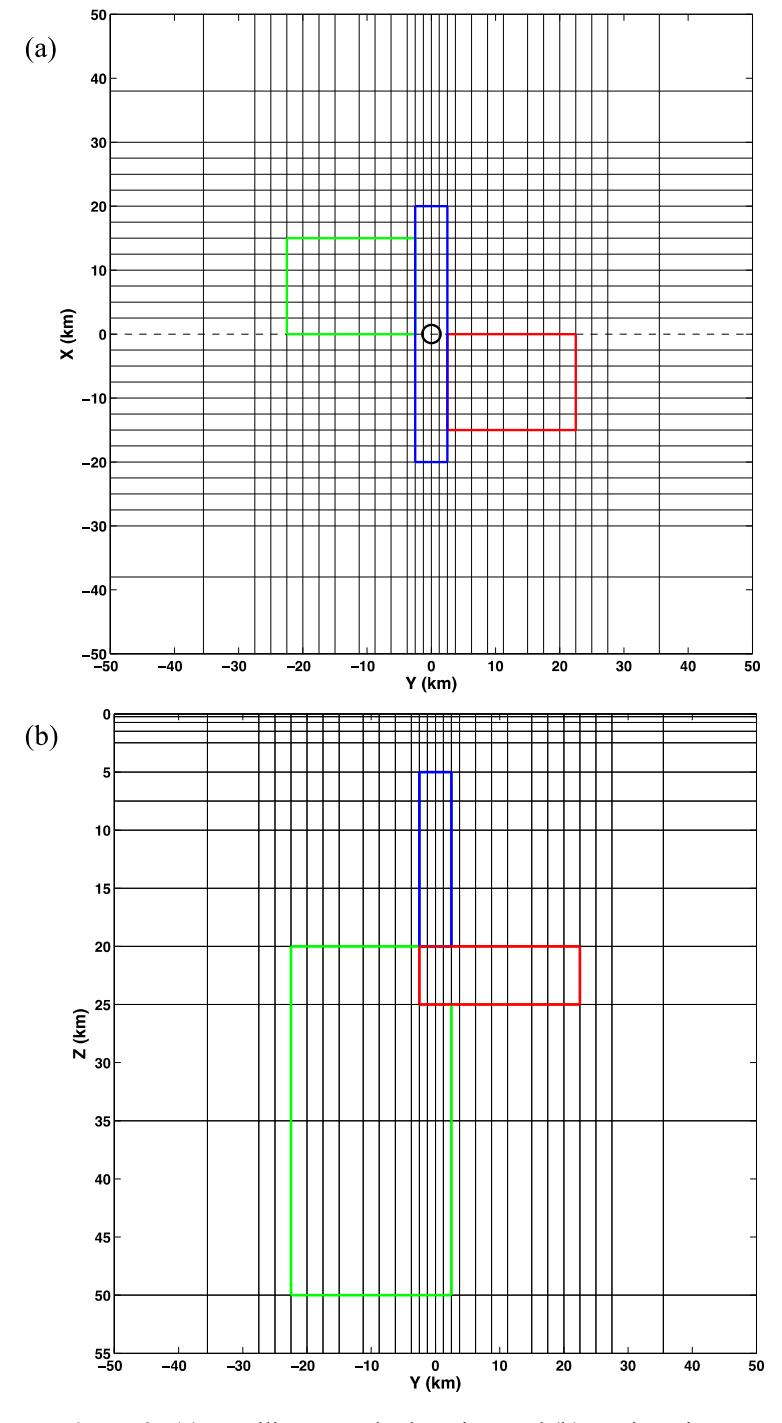
Figure 3 (a) Rectilinear mesh plan view and (b) section view.
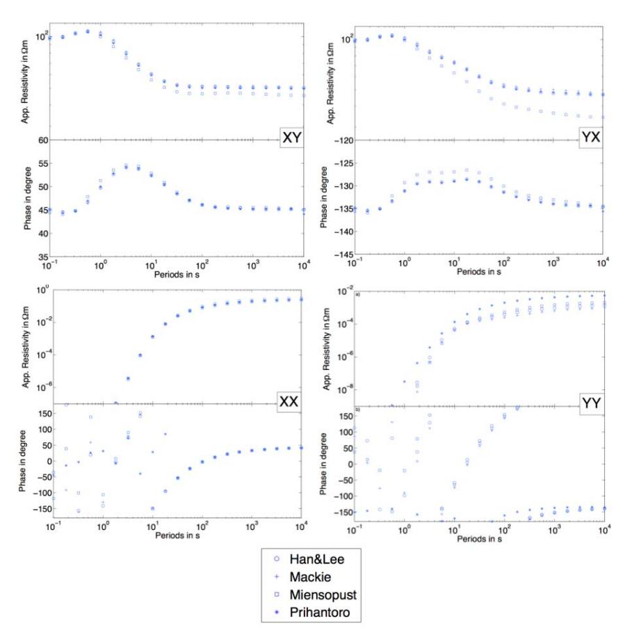
Figure 4 Comparison of the obtained DTM1 response at center site (x = y = 0 km). Apparent resistivity and phase are shown for all components XY, YX, XX and YY.
As can be seen in Figure 4, in general, all obtained response curves are in good agreement with each other. Some discrepancies can be observed in almost every response (XY, YX and YY), especially for longer periods. This is mainly due to the adopted mesh size, where some meshes are more suitable for shorter periods than for longer ones. Table 2 shows that our adopted mesh was comparable in size with the ones adopted by [23], which used FD code. However, as can be seen in Figure 4, our response was almost identical to the response given by Mackie, who adopted a much finer mesh. The finite-difference (FD) codes of [5] and [19] are basically the same since they both use a staggered grid of finite differences (SFD). In the SFD scheme implemented in [5], the continuity equation of the electric current is defined by averaging the normal electric fields across cells, which have different conductivity. Averaging is not necessary in an FE approach since the discontinuity of a normal electric field and the divergence-free condition are natural from the construction, ensuring that the electric current continuity is satisfied.
Table 2 Difference in Computation Time for Each Computer Specification Used.
| Code | Computation Time and Tolerance Target/TT (for iterative method) | Computer Specification |
|---|---|---|
| FD [5] | 30 minutes (TT: 10-10, parallel) | 36 dual processor Xeon, 3.2 GHz |
| FD [19] | 1 hour 18 minutes (TT: 10-7) | Intel Core CPU E6300, 1.86 GHz, 3.25 GB RAM |
| FE [12] | 57 hours 16 minutes (TT: 10-10) | Cluster: 256 nodes IBM x335, each 2 CPUs (Pentium IV Xeon DP 2.8 GHz) |
| FE (this work) | 5 hours 57 minutes | Laptop, 2GB RAM, Intel Core i5 1.6 GHz |
FD = finite difference, FE = finite element.
Although our approach in solving linear systems is different from the FE code in [12], the resulting response is almost identical with the response calculated by Nuree Han & Tae Jong Lee, who used the FE code from [12] with an iterative method. In [18] it is pointed out that solving linear systems using an iterative method suffers from slow convergence. As can be seen in Table 2, the slow convergence rate is reflected in the computation time needed to run the FE code from [12]. Although the computation time depends heavily on the adopted mesh and computer specifications, the FE code developed in this work requires a reasonable amount of computation time compared to the other codes.
In [18], the authors propose a divergence correction method to accelerate the convergence of their iterative solver. They also found that preconditioning is not particularly effective. It should be noted that divergence correction adds another set of equations to be solved. This is not the case when we solve the linear system using a direct method. Thus, by employing a direct method, the need to solve another equation system that arises from divergence correction can be avoided. Apart from that, the solution obtained by employing a direct method is proved to be accurate enough, as can be seen from our result.
Pseudo-sections of DTM1 along the y-axis in the center profile (dashed line in Figure 3(a)) are shown in Figure 5. The diagonal apparent resistivity values are blanked out in the pseudo-sections if the value is less than a threshold value of 10-5 Ω.m. It can clearly be seen from Figure 5(a) that the conductive bodies of DTM1 are manifested in the off-diagonal apparent resistivity where a shallow structure (body 1) exists. Meanwhile, the other structure (body 2), which is deeper as well as more conductive, is shifted to the right. Both conductive structures are buried in a roughly homogenous 100 Ω.m structure, which is the true value of the half-space background resistivity. The diagonal apparent resistivity pseudo-sections also indicate three-dimensional structures, as shown by their non-zero value. Meanwhile, the other structure in DTM1, which is highly resistive (body 3), cannot be seen in the pseudo-sections because, in general, the EM induction method is more sensitive to conductive structures.
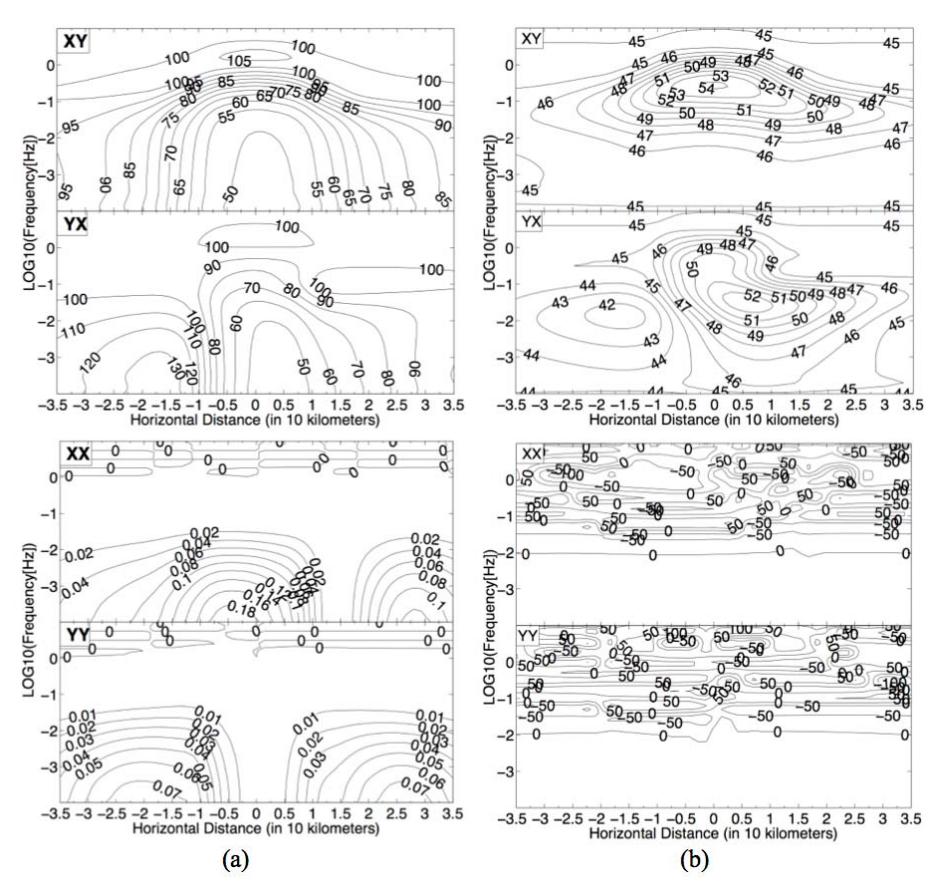
Figure 5 Pseudo-sections of DTM1 along the y-axis in the center profile, calculated using the proposed method: (a) apparent resistivity and (b) phase. Note that the diagonal element values are blanked out for resistivity if the values are less than a threshold value of 10-5 Ω.m.
6 Conclusions
Computer codes for 3-D MT forward calculation using vector finite elements with a direct method were successfully developed. The resulting 3-D MT response of the proposed codes was in good agreement with those given by other codes that use a different numerical method as well as mesh size. The approach in solving linear systems using a direct method was also seen to be comparable to other vector finite element codes using an iterative solver. The computer code developed in this work has reasonable accuracy and efficiency compared to the other codes.