
1 Introduction Compute
The resultant technique is important in elimination theory for solving systems of polynomial equations. The method has also been used to determine whether or not a set of polynomial equations has a common root without analytically or numerically solving for the roots. It can be used in many real-life and engineering applications, such as in robotics (Yang, et al. [1]), computer-aided geometric design (Lewis and Stiller [2]), geodesy and geoinformatics (Awenge et al. [3]), and many more. The resultant is figured out as a polynomial in terms of the coefficients of the given system. For the univariate system there are two types of constructions, namely the Sylvester and Bézout resultant, as respectively proposed by Sylvester [4] and Bézout [5]. The size of the Sylvester resultant matrix is large but easy to compute, while the Bézout matrix has complicated entries but produces a comparatively small-sized matrix. Macaulay
[6] and Dixon generalized the Sylvester and Bézout cases to their respective multivariate settings. Any setting that combines two methods is referred to as a hybrid resultant matrix. A detailed comparison of a number of existing hybrid methods is given by Sulaiman & Aris [7].
For a system of polynomials F f f f Kx x 12 1 , , , [ ,..., ] n n with their respective degrees 1 2 , ,..., n dd d , the classical Macaulay method of computing the resultant polynomial is given by the ratio of the two matrices. Wang & Lian [8] give the implementation of the Macaulay method for the system of three polynomial equations. One major setback of this method is that the determinants of the two matrices can be zero. In addition, Kapur & Saxena [9] gave an example that shows that the resultant cannot always be computed using the Macaulay formulation.
Jouanolou [10,11] modified Macaulay's method to produce a tighter matrix, resulting in another Macaulay-style formula. His formulation consists of four blocks. Two of the blocks are defined by some mappings that are purely Sylvester-type, while the third block is defined using a Bézoutian matrix and the final block consists of zero entries only. Szanto in [12] observed that the Jouanolou method also produces some extraneous factors and proposed a Macaulay-style formula by dividing the resultant matrix with a minor matrix, called the matrix of unwanted factors.
To determine the Bézoutian matrix of the Jouanolou method, first, the differentials are computed and arranged in the matrix using a certain order. Then the determinants of the matrix of differentials are used to determine the entries of the Bézoutian matrix, also called the Morley form [11]. The computation of the determinants usually gives very large polynomials, which makes the extraction of the entries of the Bézoutian matrix very difficult. The proposed method replaces the Bézoutian matrix with a portion of the entry formula for computing the resultant given by Chionh, et al. [13].
The Dixon formulation can produce the smallest resultant matrix. However, the entries of the Dixon matrix are complicated in comparison to other Sylvestertype methods. As an alternative to the direct method of computing the Dixon resultant matrix, two different algorithms are proposed in Chionh, et al. [13-14]. Zhao & Fu [15] extended one of the algorithms to more general form and Qin, et al. [16] gave a complexity analysis of the generalized algorithm. The algorithms compute the Dixon resultant matrix directly from the coefficients, which avoids computation of an intermediate expression swell that usually occurs during large polynomial computations [13]. Details of the resultant formulations in relation to extraneous factors can be found in [17-18]. In this paper, a hybrid method for computing the resultant matrix is proposed. The hybrid setting is based on the Dixon-Jouanolou methods. A portion of the entry formula for computing the Dixon matrix is combined with one of the mappings of the Jouanolou method.
2 Background
This section gives a brief description of the two methods considered for construction of the hybrid method. A detailed description can be found in [12-14]; these background materials are given to make this paper self-contained.
2.1 The Jouannolou Method
Consider the system of homogeneous polynomials \(F = \{f_1, f_2, ..., f_n\} \in K[x_1, ..., x_n]\) with their respective degrees given as \(d_1, d_2, ..., d_n\). The critical degree is given by:
\[\delta = \sum_{i=1}^{n} (d_i - 1) \tag{1}\]
Using Eq. (1), the size of the Jouanolou matrix is given by the formula:
\[S(M_r) = {r+n-1 \choose n-1} + \lambda(\delta - r), \qquad 0 \le r \le \delta.\] (2)
The parameter \(\lambda(\delta-r)\) is the dimension of the \(\tau\) – vector space; the size of the Jouannlou method depends on the right choice of parameter r. The elements of the \(\tau\) – vector space are of a degree \(\delta-r\) in the ideal generated by system F.
Definition 2.1 [12] Let \(F = \{f_1, f_2, ..., f_n\} \in K[x_1, ..., x_n]\) be a system of homogeneous polynomials. For \(0 \le \xi \le \delta + 1\) the following terms are defined:
\[\operatorname{Mon}_{n}(\zeta) = \{x^{\xi} : |\xi| = \zeta\}\] \[\operatorname{Rep}_{d}(\zeta) = \{x^{\xi} : |\xi| = \zeta, \ \exists i \ni \zeta_{i} \ge d_{i}\}\] \[\operatorname{Dod}_{d}(\zeta) = \{x^{\xi} : |\xi| = \zeta, \ \exists i \ne j \ \ni \zeta_{i} \ge d_{i}, \zeta_{j} \ge d_{j}\}\]
Definition 2.2 [12] Let \(f_i = \sum C_{a_i} x^{a_i} \in K[x_1, x_2, ..., x_n]\) with \(x = (x_1, x_2, ..., x_n)\) and let \(y = (y_1, y_2, ..., y_n)\) be a new variable and define the differentials \(\Delta_{i,j}(x,y)\) by \(\Delta_{i,j}(x,y) = \frac{f_i(y_1, ..., y_{j-1}, x_j, ..., x_n) - f_i(y_1, ..., y_j, x_{j+1}, ..., x_n)}{x_j - y_j}\),
\(1 \le i, j \le n\) which can be written as:
\[f_i(y_1,...,y_{j-1},x_j,...,x_n) - f_i(y_1,...,y_j,x_{j+1},...,x_n)\]
= \(\Delta_{i,i}(x,y)(x_i-y_i)\) 1 \le i, j \le n.
The Bézoutian block is computed from the following determinant:
\[\Delta(x, y) = \det(\Delta_{i, j}(x, y)(x_j - y_j))_{1 \le i, j \le n} = \sum_{|\gamma| \le \nu} \Delta_{\gamma}(x) \cdot y^{\gamma}\]
Definition 2.3 [12] For a fixed r, \(0 \le r \le \delta\), the Jouanolou resultant matrix is given by:
\[J_{r}(F) = \begin{bmatrix} \varphi_{r} & \theta_{\partial - r} \\ \theta_{r}^{*} & 0 \end{bmatrix}\] where \(\varphi_t\), \(\theta_{\partial - t}\) and \(\theta_t^*\) represent the following mappings:
\[\varphi_r :< \operatorname{Mon}(r) >^* \longrightarrow < \operatorname{Mon}(\partial - r) > \ni y^\omega \longrightarrow \operatorname{Morl}_\omega(x)\] (3)
If \(x^{\zeta} \in \operatorname{Rep}_d(r)\), then let \(i(\zeta)\) be the smallest index such that \(\zeta_{i(\zeta)} \ge d_{i(\zeta)}\) and define:
\[\theta_{\partial -r} :< \operatorname{Rep}_{d}(\partial -r) > \longrightarrow < \operatorname{Mon}(\partial -r) > \ni x^{\omega} \longrightarrow (\frac{x^{\omega}}{x_{i(\zeta)}^{d_{i(\zeta)}}}) \cdot f_{i(\zeta)}\](4)
\[\theta_{r}^{*} :< \operatorname{Mon}(r) >^{*} \longrightarrow < \operatorname{Rep}_{d}(r) > \ni y^{\omega} \longrightarrow \sum_{x^{\omega} \in \operatorname{Rep}_{d}(r)} y^{\omega} (\theta_{r}(x^{\omega})) \cdot y^{\omega}\] (5)
Definition 2.3 describes the Jouannolou resultant matrix for \(r \le \delta\), if \(r \ge \delta\) the formulation precisely gives the classical Macaulay resultant matrix.
2.2 Entry Formula
Consider the bivariate system of degree \((m_1, m_2)\). The system of Eq. (6) is assumed to be unmixed, which means they have the same set of exponents.
\[f_1 = \sum_{i=0}^{m_1} \sum_{j=0}^{m_2} a_{i,j} x^i y^j, \quad f_2 = \sum_{k=0}^{m_1} \sum_{l=0}^{m_2} b_{k,l} x^k y^l, \quad f_3 = \sum_{p=0}^{m_1} \sum_{q=0}^{m_2} c_{p,q} x^p y^q\] (6)
Let \((x_1, y_1)\) be a set of new variables. Using the Dixon method, the following determinant is given as:
\[Det(x, y, x_1, y_1) = \begin{vmatrix} f_1(x, y) & f_2(x, y) & f_3(x, y) \\ f_1(x_1, y) & f_2(x_1, y) & f_3(x_1, y) \\ f_1(x_1, y_1) & f_2(x_1, y_1) & f_3(x_1, y_1) \end{vmatrix}\](7)
Simplifying Eq. (7) gives another equation in terms of summations:
\[Det(x, y, x_1, y_1) = \sum_{i=0}^{m_1} \sum_{i=0}^{m_2} \sum_{k=0}^{m_1} \sum_{k=0}^{m_2} \sum_{n=0}^{m_1} \sum_{q=0}^{m_2} |i, j; k, l; p, q| x^i y^{j+l} x_1^{k+p} y_1^q\] (8)
Here |i, j; k, l; p, q| are the \(3 \times 3\) determinants in terms of the coefficients of the polynomials defined by Eq. (6) as given in Eq. (9):
\[\begin{vmatrix} i, j; k, l; p, q \end{vmatrix} = \begin{vmatrix} a_{i,j} & b_{i,j} & c_{i,j} \\ a_{k,l} & b_{k,l} & c_{k,l} \\ a_{p,q} & b_{p,q} & c_{p,q} \end{vmatrix}\](9)
Let a = i, c = k + p, b = j + l and d = q. Eq. (8) can be represented in the following form:
\[\operatorname{Det}(x, y, x_{1}, y_{1}) = \sum_{a=0}^{m_{1}} \sum_{b=0}^{2m_{2}} \sum_{c=0}^{2m_{1}} \sum_{d=0}^{m_{2}} C_{a,b,c,d} x^{a} y^{b} x_{1}^{c} y_{1}^{d}\] (10)
Here, \(C_{a,b,c,d}\) denotes the coefficients of \(x^a y^b x_1^c y_1^d\) in \(Det(x,y,x_1,y_1)\). Note that \(Det(x,y,x_1,y_1)\) is divisible by \((x-x_1)(y-y_1)\), therefore the Dixon polynomial is defined as:
\[\Delta(x, y, x_1, y_1) = \frac{\operatorname{Det}(x, y, x_1, y_1)}{(x - x_1)(y - y_1)} \tag{11}\]
The Dixon polynomial defined in Eq. (11) is of degree at most \(m_1 - 1\) in x, \(2m_2 - 1\) in y, \(2m_1 - 1\) in \(x_1\) and \(m_2 - 1\) in \(y_1\). Substituting Eq. (10) into Eq. (11) and a little work gives:
\[\Delta(x, y, x_1, y_1) = \sum_{a=0}^{m_1-1} \sum_{b=0}^{2m_2-1} \sum_{c=0}^{2m_1-1} \sum_{d=0}^{m_2-1} C_{a,b,c,d} x^a y^b x_1^c y_1^d\] (12)
To avoid polynomial divisions, a formula for the sum to infinity is employed so that the fraction can be written as:
\[\frac{1}{(x-x_1)(y-y_1)} = \frac{1}{xy} \sum_{u=0}^{\infty} \left(\frac{x_1}{x}\right)^{u} \sum_{v=0}^{\infty} \left(\frac{y_1}{y}\right)^{v}\] (13)
Substituting Eq. (8) and Eq. (13) into Eq. (11) gives:
\[\Delta(x, y, x_1, y_1) = \sum_{i,j;k,l;p,q} \sum_{u,v} |i,j;k,l;p,q| x^i y^{j+l} x_1^{k+p} y_1^q \frac{x_1^u}{x^{u+1}} \frac{y_1^v}{y^{v+1}}\](14)
Equating both sides of Eq. (12) and Eq. (14) gives:
\[\sum_{a,b,c,d} C_{a,b,c,d} x^{a} y^{b} x_{1}^{c} y_{1}^{d}\] \[= \sum_{i,j;k,l;p,q} \sum_{u,v} |i,j;k,l;p,q| x^{i} y^{j+l} x_{1}^{k+p} y_{1}^{q} \frac{x_{1}^{u}}{x^{u+1}} \frac{y_{1}^{v}}{y^{v+1}}\] (15)
Comparing the exponents of Eq. (15) gives:
\[i = a + u + 1, k + p = c - u, j + l = b + v + 1 \text{ and } q = d - v\] (16)
Referring back to Eq. (6), the two constraints \(0 \le i, k, p \le m_1\) and \(0 \le j, l, q \le m_2\) are found. Combining these constraints with Eq. (16) gives:
\[0 \le a + u + 1 \le m_1\], \(0 \le b + v + 1 \le 2m_2\), \(0 \le c - u \le 2m_1\) and \(0 \le d - v \le m_2\) (17)
Considering Eq. (13), the constraints \(0 \le v, u < \infty\) can be obtained and from Eq. (12). The following condition is imposed:
\[0 \le a \le m_1 - 1\], \(0 \le b \le 2m_2 - 1\), \(0 \le c \le 2m_1 - 1\) and \(0 \le d \le m_2 - 1\) (18)
Combining Eq. (16) and Eq. (17) for \(0 \le v, u < \infty\) gives another set of constraints in terms of u, v as follows:
\[0 \le u \le \min(c, m_1 - 1 - a) \text{ and } 0 \le v \le \min(d, 2m_2 - 1 - b)\] (18)
Referring to Eq. (16), the coefficients of \(C_{a,b,c,d}\) can now be written in the following form:
\[|i, j; k, l; p, q| = |a + 1 + u, b + 1 + v - l; k, l; c - u - k, d - v|\] (19)
Note that there are existing constraints \(0 \le k \le m_1\) and \(0 \le l \le m_2\) together with other constraints \(0 \le b+1+v-l \le m_2\) and \(0 \le c-u-k \le m_1\) from Eq. (16); k and l have the following conditions:
\[\max(0, c - u - m_1) \le k \le \min(m_1, c - u);\]
\[\max(0, b + 1 + v - m_2) \le l \le \min(m_2, b + 1 + v)\]
(20)
Combining Eqs. (18), Eq. (19) and Eq. (20), the first entry formula emerges:
\[C_{a,b,c,d} = \sum_{u=0}^{\min(c,m_1-1-a)\min(d,2m_2-1-b)} \sum_{k=\max(0,c-1-m_1)}^{\min(m_1,c-u)}\]
\[\sum_{l=\max(0,b+1+v-m_2)}^{\min(m_2,b+1+v)} \left| a+1+u,b+1+v-l;k,l;c-u-k,d-v \right|\] (21)
Note that getting rid of the intermediate cancelling terms, which are precisely in the range of l from 0 to d, Eq. (21) can be improved as follows:
\[C_{a,b,c,d} = \sum_{u=0}^{\min(c,m_1-1-a)} \sum_{v=0}^{\min(d,2m_2-1-b)} \sum_{k=\max(0,c-1-a)}^{\min(m_1,c-u)}\] \[\sum_{l=\max(b+1,b+1+v-m)}^{\min(m_2,b+v-d)} |a+1+u,b+1+v-l;k,l;c-u-k,d-v|\] (22)
The formula given in Eq. (22) first appeared in [13], providing a systematic way of computing the entries of the Dixon resultant matrix.
3 Main Results
This section introduces the hybrid construction that combines the mapping defined in Eq. (4) with the entry formulation given by Eq. (22). The hybrid matrix consists of four blocks: the first block is defined by Eq. (22), the second and third blocks are given by Eq. (4), while the final block consists of zero entries only.
3.1 Hybrid Formulation
Definition 3.1 Let \(r \ge 0\) be a fixed parameter; the resultant matrix of the system of polynomials \(F = \{f_1, f_2, ..., f_n\} \in K[x_1, ..., x_n]\) is contained in the determinant of the following matrix:
\[\mathbf{R}_{r}(F) = \begin{bmatrix} A & C \\ C^{T} & 0 \end{bmatrix}.\]
Eq. (22) is used to compute the entries of block A with the following additional conditions:
\[\begin{cases} 0 \le u, v < \infty \\ 0 \le a, d \le \left\lfloor \frac{1}{2} \max(m_1, m_2) \right\rfloor, \\ 0 \le b, c \le \max(m_1, m_2) \end{cases}\] where the function \(\lfloor \ \rfloor\) denotes the floor function.
The entries of block \(\mathcal{C}\) and its transpose are computed from Eq. (4), subject to the following condition:
\[r = \left| \begin{array}{c} \sum_{i=1}^{n} \left( d_{i} - 1 \right) \\ \hline 2 \end{array} \right| .\]
Let \(d_{\max} = \max(d_1, d_2, \dots, d_n)\), where each \(d_i\) denotes the degree of \(f_i\), the size of the hybrid matrix is estimated by the formula:
\[S(R_r) \le (n-1)! \times d_{\max} + \rho . \tag{23}\]
Here \(\rho = |Rep(r)|\) denotes the number of multipliers found in the sets of monomials Rep(r). These multipliers are used to obtain the entries of block C as well as \(C^T\).
Notice the Dixon resultant requires the system to have n+1 polynomials with n variables. Geometrically speaking the results are considered to be in an affine space. However, the Jouanolou method requires n+1 polynomials with n+1 variables, which define a projective resultant. To overcome the different requirements of these methods, the notion of pseudo-homogenization is introduced.
3.2 Pseudo-homogenization
Definition 3.2 A variable \(x_m\) is called an artificial variable if it satisfies the following conditions:
- 1. \(x_{m}^{n} = 1\) for \(n \in \mathbb{N}\)
- 2. 2. For all \(n \in \mathbb{N}\) \(x_m = x_m^2 = \cdots = x_m^n\).
Definition 3.3 Pseudo-homogenization is the act of using an artificial variable to normalize the system of polynomial equations from inhomogeneous to homogeneous and vice versa.
Example 1 Let F be a system of polynomials in the variables x, y:
\[F = \begin{cases} f_1 = 4x^2 + 5x + 6y^2 + 3ay + 5y + 1 \\ f_2 = 5x^2 + xy + 2ax + 6a^2 + 3a + 3 \\ f_3 = 6ax + 5y^2 + 2y + 4a^2 + 6a + 5 \end{cases}\] (24)
Using Definitions 3.2 and 3.3, a pseudo-variable z can be used to homogenize the system of Eq. (24) into the following form:
\[F = \begin{cases} f_1 = 4x^2 + 5xz + 6y^2 + 3ayz + 5yz + z^2 \\ f_2 = 5x^2 + xy + 2axz + (6a^2 + 3a + 3)z^2 \\ f_3 = 6axz + 5y^2 + 2yz + (4a^2 + 6a + 5)z^2 \end{cases}\](25)
Note that the hybrid method uses the two forms described in Eqs. (24) and (25). The entry formula requires that the system is inhomogeneous, while the mapping defined in Eq. (4) requires a homogeneous system.
Figure 1 describes the procedure for computing the hybrid resultant matrix. The system of equations can be either homogeneous or inhomogeneous. In whatever case, the notion of pseudo-homogeneousness will be used to homogenize or dehomogenize the equations based on the conditions of the individual block.
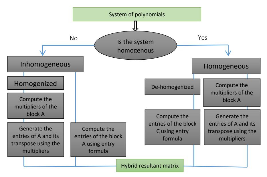
Figure 1 Procedure for computing the hybrid resultant matrix.
3.3 Elements of the Entry Formula
This section describes the elements of the entry formula given in Eq. (22). Referring to the system of polynomial equations given by Eq. (6), the direct method for computing the Dixon resultant matrix is given by the formula:
\[\Delta(x,y,\alpha,\beta) = \frac{1}{(\alpha-x)(\beta-y)} \begin{vmatrix} f_1(x,y) & f_2(x,y) & f_3(x,y) \\ f_1(\alpha,y) & f_2(\alpha,y) & f_3(\alpha,y) \\ f_1(\alpha,\beta) & f_2(\alpha,\beta) & f_3(\alpha,\beta) \end{vmatrix}\](26)
Where \(\alpha\) and \(\beta\) are regarded as new variables. By means of a lexicographical order x > y and \(\alpha > \beta\) as imposed in [14], the following system can be obtained:
\[\text{[rumus tidak dapat ditampilkan dengan baik — lihat PDF asli]}\]
Here, D is the Dixon resultant matrix and Eq. (28) gives the complete nature of the elements of the Dixon matrix:
\[D = \begin{bmatrix} C_{0,0,0,0} & C_{0,0,0,1} & \cdots & \cdots & C_{0,0,2s-1,t-1} \\ C_{0,1,0,0} & & & & C_{0,1,2s-1,t-1} \\ \vdots & & \ddots & & & \vdots \\ \vdots & & & & \ddots & \vdots \\ C_{s-1,2t-1,0,0} & C_{s-1,2t-1,0,1} & \cdots & \cdots & C_{s-1,2t-1,2s-1,t-1} \end{bmatrix}\] \[(28)\]
Note that the elements of matrix D are computed directly from Eq. (22) such that the computation can be performed in parallel. Example 2 shows that the computation of each entry is independent.
\[D = \begin{bmatrix} C_{0,0,0,0} & C_{0,0,0,1} & C_{0,0,1,0} & C_{0,0,1,1} & C_{0,0,2,0} & C_{0,0,2,1} & C_{0,0,3,0} & C_{0,0,3,1} \\ C_{0,1,0,0} & C_{0,1,0,1} & C_{0,1,1,0} & C_{0,1,1,1} & C_{0,1,2,0} & C_{0,1,2,1} & C_{0,1,3,0} & C_{0,1,3,1} \\ C_{0,2,0,0} & C_{0,2,0,1} & C_{0,2,1,0} & C_{0,2,1,1} & C_{0,2,2,0} & C_{0,2,2,1} & C_{0,2,3,0} & C_{0,2,3,1} \\ C_{0,3,0,0} & C_{0,3,0,1} & C_{0,3,1,0} & C_{0,3,1,1} & C_{0,3,2,0} & C_{0,3,2,1} & C_{0,3,3,0} & C_{0,3,3,1} \\ C_{1,0,0,0} & C_{1,0,0,1} & C_{1,0,1,0} & C_{1,0,1,1} & C_{1,0,2,0} & C_{1,0,2,1} & C_{1,0,3,0} & C_{1,0,3,1} \\ C_{1,1,0,0} & C_{1,1,0,1} & C_{1,1,1,0} & C_{1,1,1,1} & C_{1,1,2,0} & C_{1,1,2,1} & C_{1,1,3,0} & C_{1,1,3,1} \\ C_{1,2,0,0} & C_{1,2,0,1} & C_{1,2,1,0} & C_{1,2,1,1} & C_{1,2,2,0} & C_{1,2,2,1} & C_{1,2,3,0} & C_{1,2,3,1} \\ C_{1,3,0,0} & C_{1,3,0,1} & C_{1,3,1,0} & C_{1,3,1,1} & C_{1,3,2,0} & C_{1,3,2,1} & C_{1,3,3,0} & C_{1,3,3,1} \end{bmatrix}\]
Example 2 Let the degree of the system of Eq. (6) be \(m_1 = m_2 = 2\), the Dixon resultant matrix will be a square matrix of dimensions \(2m_1m_2\) as described by Eq. (28). The entry \(C_{0.1,0.1}\) can be computed using Eq. (22) as follows:
\[C_{0,1,0,1} = \sum_{u=0}^{1} \sum_{v=0}^{1} \sum_{k=1}^{1} \sum_{l=2}^{1} |1, v; 2, 0; 0, 1-v| + \sum_{u=0}^{1} \sum_{v=0}^{1} \sum_{k=1}^{1} \sum_{l=2}^{1} |1, v; 0, 2, 1, 1-v|\]
\[C_{0,1,0,1} = \left|1,0;1,2;0,1\right| + \left|1,1;1,2;0,0\right| + \left|1,0;0,2;1,1\right| + \left|1,1;0,2;1,0\right|\] where each |i,j;k,l;p,q| is a \(3 \times 3\) determinant and they are computed using Eq. (9). Note that computing each entry largely depends on the values of a,b,c and d in \(C_{a,b,c,d}\). The values a,b,c and d have unique combinations that allow parallel computation of the entries.
In Example 3, we use a system of three polynomial equations of degree at most two to describe how this hybrid method can be used to compute the resultant polynomial.
Example 3 Consider the system of homogeneous polynomials in \(x_1, x_2, x_3\):
\[F = \begin{cases} f_1 = a_1 x_1 + a_2 x_2 + a_3 x_3 \\ f_2 = b_1 x_1 + b_2 x_2 + b_3 x_3 \\ f_3 = c_1 x_1^2 + c_2 x_2^2 + c_3 x_3^2 + c_4 x_1 x_2 + c_5 x_1 x_3 + c_6 x_2 x_3 \end{cases}\]
Since the given system is homogenous, the two blocks C and \(C^T\) are computed as follows:
\[\delta = \sum_{i=1}^{3} (d_i - 1) = 1, \ r = \left\lfloor \frac{\delta}{2} \right\rfloor = 0 \text{ and } \operatorname{Rep}(\delta - r) = \operatorname{Rep}_{(1,1,2)}(1) = \{x_1, x_2\}.\]
Using the mapping defined in Eq. (4), the multipliers are found and the blocks C and \(C^T\) are computed.
To compute block C, the system is dehomogenized by setting \(x_3 = 1\) and the entry formula is used for the computation of the block according to Definition 3.1. Combining the four blocks together, the following is the \(5 \times 5\) resultant matrix for the system in Example 3:
\[\begin{bmatrix} a_1b_2c_3 - a_1b_3c_6 - a_2b_1c_3 + a_2b_3c_5 + a_3b_1c_6 - a_3b_2c_5 & a_3b_1c_2 - a_1b_3c_2 & a_2b_3c_1 - a_1b_3c_4 + a_3b_1c_4 - a_3b_2c_1 & a_1 & b_1 \\ a_2b_3c_4 - a_1b_3c_2 + a_3b_1c_2 - a_3b_2c_4 & a_2b_1c_2 - a_1b_2c_2 & a_2b_1c_4 - a_1b_2c_4 & a_2 & b_2 \\ a_2b_3c_1 + a_3b_2c_1 & 0 & a_2b_1c_1 - a_1b_2c_1 & a_3 & b_3 \\ a_1 & a_2 & a_3 & 0 & 0 \\ b_1 & b_2 & b_3 & 0 & 0 \end{bmatrix}\]
The determinant of the above matrix is the projection operator. If the determinant is an irreducible polynomial in terms of the coefficients of the given system, then it is considered exact.
4 Complexity Analysis
This section presents the computational analysis of the Dixon-Jouanolou method. The hybrid method has two components, called Sylvester and Bézout type. The monomial Rep(r) is used to generate one of the Sylvester parts while \(Rep(\delta - r)\) is used to obtain the other. However, a loose entry formula is used obtained the Bézout block. Referring to Eq. (22), two factors need to be considered:
i. The precise number of \(3 \times 3\) determinants required.
ii. The estimated number of multiplications and additions necessary while computing each determinant.
Referring to Eq. (22) for a bivariate case, Chionh, et al. in [14] estimate the upper bound of the \(3 \times 3\) determinants as:
\[C^{m_1, m_2} \le \frac{m_1^2 (m_1 + 1)(2m_1 + 1)m_2^2 (m_2 + 1)(m_2 + 2)}{3}\] (29)
where \(m_1\) and \(m_2\) are the highest exponents of \(x_1\) and \(x_2\) respectively. Eq. (29) provides only the estimate of the number of \(3 \times 3\) determinants. For bivariate systems the exact number of \(3 \times 3\) determinants is estimated by Eq. (30):
\[D^{m_1,m_2} = \frac{m_1(m_1+1)^2(m_1+2)}{6} \times \frac{m_2(m_2+1)^2(m_2+2)}{6}\] (30)
Eq. (30) was obtained by Chionh, et al. [14] for \(m_1 = m_2 = 2\) after solving 25 linear equations in terms of the coefficients of the three bivariate equations. Proposition 1 gives the computational cost of computing the Dixon resultant using an entry formula.
Proposition 1. The computational complexity of formulating the Dixon resultant matrix using the loose entry formula described by Eq. (22) for bivariate systems requires \(O(m_1^3 m_2^3)\) multiplications and additions.
Proof: Referring to Eq. (22), the number of \(3 \times 3\) determinants is given by Table 1.
Table 1 Exponents of the Polynomials and their Corresponding Number of Determinants.
| \((m_1,m_2)\) | Number 3 × 3 Determinants |
|---|---|
| (1,2) | 36 |
| (2,2) | 144 |
| (5,7) | 26460 |
| (10,15) | 1346400 |
| (20,17) | 13430340 |
From Table 1, Eq. (30) is derived only for (2,2), which gives 144 determinants. Apart from that, Eq. (30) fails to provide the exact number. Modifying Eq. (30) to a more general setting gives the following equation:
\[E^{m_1, m_2} = \frac{m_1(m_1 + 1)^2(m_1 + 2)}{n(m_1 + 1)} \times \frac{m_2(m_2 + 1)^2(m_2 + 2)}{n(m_2 + 1)}\](31)
Note that \(m_1\) and \(m_2\) stand for the highest power of variables \(x_1\) and \(x_2\) respectively from the bivariate system. The perimeter n represents the number of variables. Simplifying Eq. (31) gives:
\[E^{m_1, m_2} = \frac{m_1(m_1 + 1)(m_1 + 2)m_2(m_2 + 1)(m_2 + 2)}{4}\] (32)
To compute each \(3 \times 3\) determinant, 12 multiplications and 5 additions are required. Therefore, the total number of multiplications and additions required is estimated by Eq. (33):
\[\begin{cases} 3m_1(m_1+1)(m_1+2)m_2(m_2+1)(m_2+2) & \text{multiplications} \\ \frac{5}{4}m_1(m_1+1)(m_1+2)m_2(m_2+1)(m_2+2) & \text{addditions} \end{cases}\] (33)
Expanding the terms of Eq. (33) gives \(O(m_1^3 m_2^3)\) multiplications and additions respectively.
The second part of the hybrid method consists of the Sylvester part. The formula \(N_{(monomials)} = \frac{1}{2}(m_1 + m_2 + 1)(m_1 + m_2 + 2)\) is used to estimate the number of monomials available in each homogeneous polynomial in three variables. There are at least n monomial multipliers for each polynomial equation. Therefore, a system of three bivariate polynomials requires the following operations:
\[\begin{cases} \frac{3n}{2}(m_{_{1}} + m_{_{2}} + 1)(m_{_{1}} + m_{_{2}} + 2) & \text{multiplications} \\ \frac{3}{2}((m_{_{1}} + m_{_{2}} + 1)(m_{_{1}} + m_{_{2}} + 2) - 1) & \text{additions} \end{cases}\](34)
So if we compute all these \(3 \times 3\) intermediate determinants just once and store them, we need to perform at least
\[\begin{cases} 3m_1(m_1+1)(m_1+2)m_2(m_2+1)(m_2+2) + 2\left[\frac{3n}{2}(m_1+m_2+1)(m_1+m_2+2)\right] \\ \text{multiplications} \end{cases}\] \[\begin{cases} \frac{5}{4}m_1(m_1+1)(m_1+2)m_2(m_2+1)(m_2+2) + 2\left[\frac{3}{2}((m_1+m_2+1)(m_1+m_2+2)-1)\right] \\ \text{additions} \end{cases}\]
Therefore the complexity of the Dixon-Jouanolou resultant matrix involves \(O(m_1^3 m_2^3)\) multiplications and \(O(m_1^3 m_2^3)\) additions.
Chionh [14] reported that the computational cost of constructing the Dixon resultant matrix entails \(O(m_1^4m_2^4)\) multiplications and \(O(m_1^4m_2^4)\) additions. A summary of the complexity of computing the entries of the Dixon resultant matrices are given in Table 2. The result of the analysis shows an improvement in terms of the complexity of computing the polynomials resultant using the new hybrid method. This analysis is done without the application of parallel computation, which can further pick up the performance of the Dixon-Jouanolou method.
Table 2 Complexity for Computing Standard Dixon versus Hybrid Method.
| Types of Operation | Standard Dixon Method | New Hybrid Method |
|---|---|---|
| Multiplications | \(0(m_1^4m_2^4)\) | \(0(m_1^3m_2^3)\) |
| Additions | \(O(m_1^4 m_2^4)\) | \(O(m_1^{\bar{3}}m_2^{\bar{3}})\) |
5 Conclusion
This paper presented a new approach of computing the resultant polynomial from a given system of equations; this notion is used for solving systems of multivariable polynomials. The efficiency of the matrix method depends on the size of the matrix and the nature of the elements of the resultant matrix. A new approach of computing the entries of the hybrid resultant matrix was presented in addition to producing a smaller matrix compared to existing hybrid methods, such as the Sylvester-Bézout hybrid formulation [19], the Cayley-Sylvester hybrid method [14] and the Sylvester-Cayley hybrid formulation [14].
Acknowledgements
This work was supported by Universiti Teknologi Malaysia under the Research University Grant, GUP vet 12J30, and Ministry of Higher Education Malaysia and UTM International Doctoral Fellowship (UTM-IDF).