1 Introduction

The main challenge in all geophysical methods, including gravity modeling, is reconstruction of the subsurface distribution of physical parameters based on data observed on the surface. Gravity inversion is aimed at obtaining information for creating a subsurface model of the density distribution using a measured gravity acceleration, called the gravity anomaly. The gravity inversion method has been used for example to identify fracture zones [1], to monitor magma chamber deformations [2], and to perform data interpretation in ore exploration [3-8]. Due to its inherent ambiguity, underdetermined algebraic formulation and sensitivity to measurement errors, gravity inversion has the potential of producing non-unique and ill-posed solutions. To overcome these drawbacks, a prior information is often imposed on the inversion scheme to obtain feasible solutions.

In a two-dimensional (2D) domain, with the restriction that the shape and size of each cell comprising the domain are kept constant and with the assumption that the density of each cell is also constant, the associated inverse problem is linear.

Compact gravity inversion [7,9] is regarded by many as a milestone in the development of gravity interpretation. It is a stable iterative inversion that maximizes the compactness of the causative body or minimizes the volume. This method is classified as a linear inversion method, where the imposed weights are changed while the iteration is in process. Barbosa and Silva [10] improved the compact inversion scheme into a generalized compact gravity inversion to allow the compactness to be distributed along symmetry axes using Tikhonov's regulation, invoking the Guillen and Menichetti method [11] to ensure the minimum moment of inertia condition for the source. The generalized compact gravity inversion is a linear inversion with the addition of model updating and weights to the data.

Silva and Barbosa [12] proposed the so-called interactive inversion, which modifies the minimum moment of inertia requirement by adding information of the symmetry axis of the anomaly. The algorithm of interactive inversion uses the solution of under-determined cases with addition of a damping factor (λ). Ekinci [13] performed gravity inversion using the compact method employing Talwani equation [1] based forward modeling with addition of a condition to stop the iteration process.

To overcome the ill-posed linear gravity inversion problem, an L-curve approach to estimate the regularization parameter and a generalized cross validation (GCV) method have been suggested by Vatankhah, et al. [3]. Applications of minimum distance, smoothness, and compactness constraints were performed by Vatankhah, et al. [14]. Also, Grandis and Dahrin [15] proposed minimization of the moment inertia of the causal anomalous object with respect to the axes of mass concentration.

Non-linear inversion of gravity data using a global approach has been done, but the causative models are still limited to simple and fixed geometries such as dykes, spheres, cylinders, and thin sheets [5,16,17], where the number of model parameters is usually smaller than 10, i.e. lower than the number of data (overdetermined problem). In this study, we propose a linear inversion of gravity data using a global approach in the form of Very Fast Simulated Annealing (VFSA) for under-determined problems where there are more model parameters than observed data.

2 Forward Modeling and Inversion

2.1 Forward Modeling

The forward modeling formulation to calculate gravity anomalies caused by a discretized two-dimensional continuous body used in this study is based on the work of Talwani, et al. [1] as modified by Blakely [18]:

\[g = 2\gamma \rho \sum_{n=1}^{N} \frac{\beta_n}{1 + \alpha_n^2} \left[ \log \frac{r_{n+1}}{r_n} - \alpha_n (\theta_{n+1} - \theta_n) \right]\] (1)

where g is the gravity anomaly at an observation point, \(\gamma\) is the gravity constant (6.673 x 10^-11 Nm²kg^-2), \(\rho\) is the density of the rocks, and \(\theta_n\) is the angle between \(r_n\) (the line from the observation point to a point source) and the horizontal (see Figure 1). \(\alpha_n\) and \(\beta_n\) are geometry factors that are expressed by:

\[\alpha_n = \frac{x_{n+1} - x_n}{z_{n+1} - z_n} \tag{2}\] and

\[\beta_n = x_n - \alpha_n z_n \tag{3}\] where \(x_n\) and \(z_n\) are the horizontal and vertical distance from the observation point to the source point, respectively.

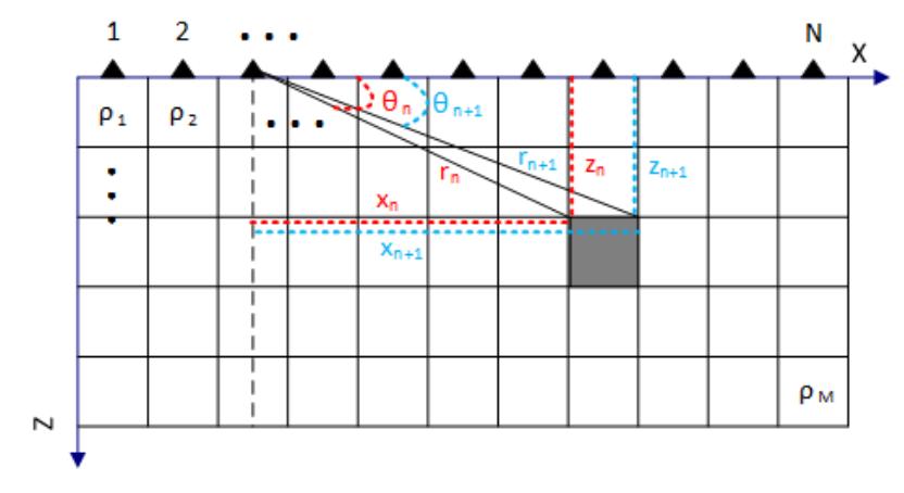
Figure 1 Illustration of the subsurface model and notations used for calculating the gravity anomaly at the surface.

Eq. (1) can be expressed in matrix notation as:

\[Gm = d (4)\] where \(\mathbf{d}\) is an \(N \times I\) data matrix, \(\mathbf{m}\) is an \(M \times I\) model parameter matrix, and \(\mathbf{G}\) is an \(N \times M\) kernel matrix or the forward operators that explicitly control the relation between \(\mathbf{d}\) and \(\mathbf{m}\). N is the total number of data and M is the total number of model parameters.

Generally, the root mean squared error (RMSE) is used as a fitness measure between observed data and calculated data:

\[RMSE = \frac{1}{N} \sqrt{\sum_{i=1}^{N} \left( \frac{G(m)_{i} - d_{i}}{\sigma_{i}} \right)^{2}}\] (5)

where \(\sigma_i\) is the standard data deviation of the i-th element of the data. The stopping criteria for inversion are the RMSE minimum value and the maximum iteration number. In our VFSA inversion, the RMSE expressed by Eq. (5) is regarded as the objective function to be minimized during the iteration process.

2.2 Very Fast Simulated Annealing Inversion

An example of a global method is simulated annealing (SA). SA inversion is analogous to the thermodynamic process of crystalline formation of a substance. At high temperatures, a liquid substance undergoes a slow cooling process causing the formation of crystals associated with a minimum energy system. From the point of view of geophysical inversion, the cooling process of temperature represents an iteration process, the substance represents a model, and the energy of the system represents an objective function. During iteration, the model will continue to converge toward a solution whose objective function is minimum.

The SA method incorporates the Boltzmann probability distribution. The distribution describes the relationship between the probability of a model m at temperature T whose energy is

\[E: P(m) \propto \exp(-\frac{E(m)}{kT}) \tag{6}\] where k is Boltzmann's constant and the system configuration is expressed in M parameters \((m_1, m_2, ..., m_M)\).

In the inversion problem, m in Eq. (6) is the model parameter, E is the objective function or misfit to be minimized, and T is a fixed control factor, commonly referred to as the iterative process controller. Since k is a constant, we can always set its value to 1 without loss of generality. Model perturbation is an important aspect in SA. It is intended to explore the model space using a directed random search.

Very Fast Simulated Annealing (VFSA) was first introduced by Ingber [19,20]. It is a modification of the SA method that was done for several reasons [21]: firstly, in an M dimension model space, each model parameter has a different range of variations and each model parameter can affect the function of misfit or energy in different ways. Therefore, each of them must have different levels of interference from their current position. Secondly, although the SA method was a breakthrough in global approaches, its algorithm is not sufficiently precise and fast to calculate if the number of Cauchy random numbers is the same as the number of model parameters. The effort of determining an M-dimensional Cauchy distribution can be averted by using the M-product of one-dimensional Cauchy distributions. Ingber [20] has proposed a new probability distribution for generating new models that depends on temperature changes.

The procedure for choosing the best model in the VSFA method can be described as follows. The first step is to generate a random initial model \((\mathbf{m}^k)\) that ranges from the minimum to the maximum model according to:

\[m_i^k = m_i^{\min} + r_i (m_i^{\max} - m_i^{\min}) \tag{7}\] where \(r_i\) is a random value between 0 and 1 and \(m_i^{\min} \le m_i^k \le m_i^{\max}\). The next step is searching for the updated model using the following rule [19]:

\[m_i^{k+1} = m_i^k + y_i (m_i^{\max} - m_i^{\min})\] (8)

where \(y_i\) is given by:

\[y_{i} = \operatorname{sgn}(u_{i} - 0.5) T_{k} \left[ \left( 1 + \frac{1}{T_{k}} \right)^{|2u_{i} - 1|} - 1 \right]\] (9)

with \(u_i \in [0,1]\).

The last step is implementation of the rule for temperature cooling, which follows

\[T_{k+1} = T_k \exp\left(-c_k k^{1/M}\right),\] (10)

where \(T_k\) is the temperature at the k-th iteration, \(T_{k+1}\) is the temperature at the k+1-th iteration and \(c_k\) is the parameter controlling the decrease of temperature. In this study, \(c_k = 1\); \(T_0 = 1\); the temperature change is taken every 20 iterations [16]. The initial model is determined using a constraint applied to the linear inversion scheme proposed by Mendonca and Silva [22,23]:

\[m = G^{T} D [DGG^{T} D + \lambda I]^{-1} Dd\] (11)

where \(\lambda = 0.1\) and is an \(N \times N\) diagonal normalization matrix:

\[D_{ii} = \left[ \sum_{j=1}^{M} G_{ij}^{2} \right]^{-1/2}. \tag{12}\]

As stated above, the objective function to be minimized in this study is given by Eq. (5). The RMSE is slightly different from the functions previously used by other authors, for example Biswas [5]. This objective function was chosen because of its practicality from an interpretation point of view since it is directly expressed in terms of fraction or percentage.

3 Results and Discussion

The modeling domain is discretized into 20 x 10 blocks (M = 200). The size of each block is 50 x 50 meter. The number of data points generated by the forward modeling scheme is 20.

Two simple test models were used. The first was a horizontal anomalous body whose contrast density was 1 gr/cm³ embedded in a background host whose contrast density is 0 g/cm³. The second test model was a vertical model whose contrast density values were the same as those of the first. These models were the same as the models used by Grandis and Dahrin [15] in their work on constraining a 2D gravity inversion by using the explicit positions of the axes of an anomalous body. The geometry of the test models is depicted by the dashed rectangular in Figures 2 and 3. Ten percent random noise was added to the generated synthetic data from both test models. The VFSA inversion for the first model imposed the assumed axis of symmetry at x = 500 m and for the second model at y = 250 m. The range of the minimum and maximum initial models was bounded between 0 and 0.5 g/cm³. The minimum-maximum range was known from the execution of Eq. (11). When the models were located around the assumed axis, then \(m^{\min} = 0\) g/cm³ and \(m^{\max} = 1\) g/cm³, and when they were far from the axis, then \(m^{\min} = 0\) g/cm³ and \(m^{\max} = 0.5\) g/cm³.

Although both of these inversions were given some constraints, the inversion solution still did not exhibit the same results as the actual models (see Figures. 2 and 3). To improve the fitness between the test models and the inverted models, specific constraints were added to the inversion schemes. For the first model, the vertical axis was kept between x = 200 m and x = 750 m, while the horizontal axis was kept at y = 250 m. In a real situation, these values may represent the constraints from a geological study. For the second model, the vertical axis was kept at x = 500 m and the horizontal axis was bounded between y = 50 m and y = 450 m. For areas within the specific constraints, models were sought between \(m^{\min} = 0.35\) g/cm³ and \(m^{\max} = 1.5\) g/cm³, while for areas outside the constraints they were sought between m min = 0 g/cm3 and mmax = 0.5 g/cm3 .

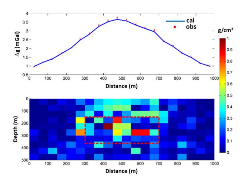
Figure 2 VFSA inversion for synthetic data generated by the first (horizontal) model. The dashed red box shows the actual test model.

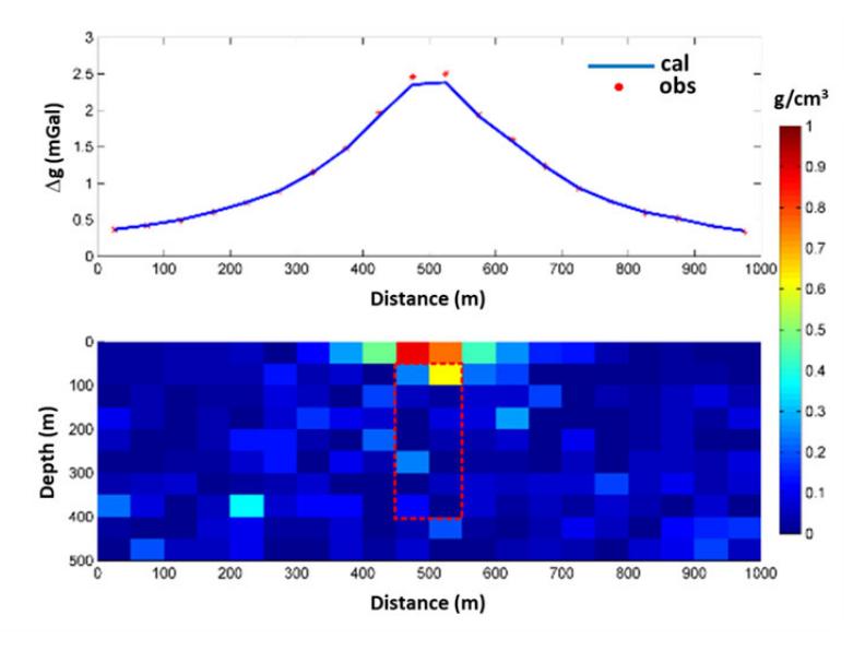
Figure 3 VFSA inversion for synthetic data generated by the second (vertical) model. The dashed red box shows the actual test model.

The advantages of VFSA inversion are its capability to give a solution that indicates the presence of the causative body and its robustness to noise embedded in the data, as can be seen from the inverted models (see Figures. 2, 3, 4(a) and 4(b)).

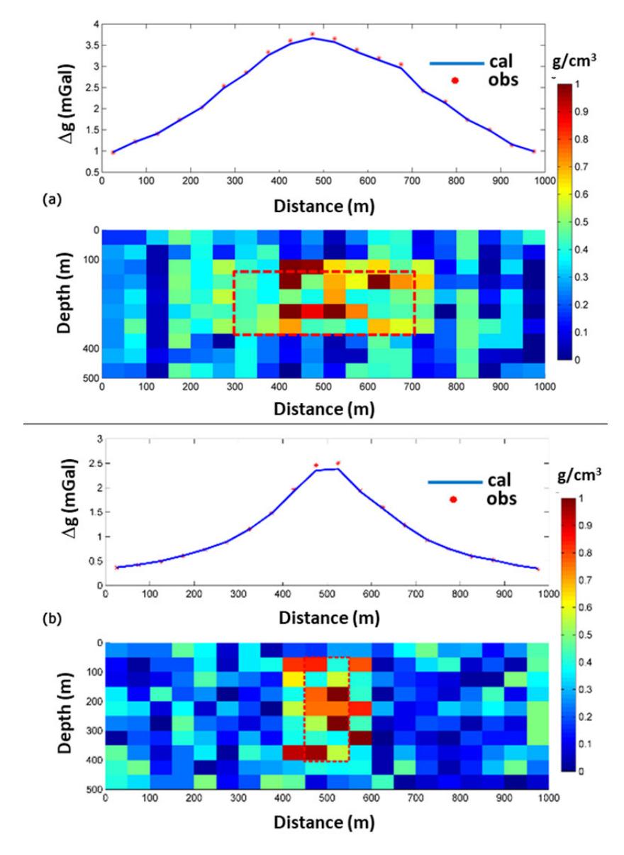
Figure 4 VFSA inversion with specific constraints for (a) the first model and (b) the second model.

However, the VFSA inversion still does not reveal geometrical constraints that are very close to those of the test models. Other examples of inversion results in which the test models cannot be fully recovered using a global approach can be found in Jin and Tao [24], who tried to address a linear 2D geomagnetic inverse problem. Nevertheless, their results indicated better recovery of the test models since they used fewer model parameters compared to this study. A seemingly better recovery of the test models for another linear 2D geomagnetic inversion using a global approach was achieved by Liu, et al. [25] using K-means clustering for constraining the model parameters.

The number of model parameters is far higher than the number of data. This affects the stability of model parameter randomness and the ambiguity of the revealed model for the given constraints in the inversion. Furthermore, the VFSA inversion requires long computational time because of the slow decrease of minimum temperature. Nevertheless, it has low possibility to be trapped in a local minimum, as can be observed from the continuously decreasing RMSE as the iteration progressed (Figure 5). The maximum iteration numbers for inversion of the horizontal and the vertical model were 3000 and 4000 respectively.

Figures 5(a) and 5(b) depict the values of RMSE and temperature of the horizontal and the vertical model for cases without application of the specific constraints where the RMSE values decrease rapidly after the 100^th iteration and reach values below 0.02 and 0.04 respectively at the 3000^th iteration. On the other hand, incorporation of specific constraints to the inversion scheme yields a better closeness between the test models and the inverted ones (Figures 4(a) and 4(b)). However, the RMSE values for the latter cases are constricted to higher values (about 0.16 for the first model and 0.18 for the second model), as can be seen from Figures. 5(c) and 5(d).

The VFSA inversion was applied to a profile of residual anomaly gravity in order to evaluate the applicability of this scheme to real data. Following Last and Kubik [9], data measured by Templeton [26] from the Woodlawn ore body situated in southeastern area of New South Wales, Australia were used. A gravity profile called Line K was used with the distance between the two gravity stations at 30.5 m (Figure 6(a)). The area contains a massive sulphide deposit at shallow depths and a copper mineralization deposit at greater depths. Briefly, the ore body can be ascribed to a copper-lead-zinc deposit produced by volcanic activity rooted in volcanic host rocks [26].

The modeling domain was discretized into 11 x 11 boxes, with the dimensions of each box at 30.5 x 30.5 m² (Figure 6(a)). The density contrast between the anomalous target (sulphide deposit) and the host rock was set to 1000 kg/m³. The specific constraints were applied using \(\lambda = 0.001\) after several tests and the number of iterations was set to 2000. The values of the inverted density contrast are shown by colors filling the boxes. A box in the i-th row and j-th column is indicated as boxi,j. The presence of high density contrasts at box7,1, box8,1 and box9,1 are in accordance with the existence of massive sulphide capped by gossan at the surface dipping into the subsurface [26], as indicated by the solid red lines in Figure 6(a). This result is in accordance with that of the compact gravity inversion by Last and Kubik [9]. However, the VFSA inversion also revealed high contrast density at box10,1 which may be attributed to the presence of an ore body surrounded by rock of lower density.

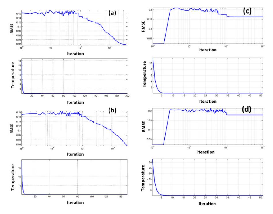
Figure 5 (a) and (b) are the VFSA inversion parameters (RMSE and temperature) of the first and the second models in Figure 2 and Figure 3, respectively, when using no specific constraints. Meanwhile, (c) and (d) are the RMSE and temperature of the first and the second model in Figure 4(a) and Figure 4(b), respectively, when using the specific constraints.

The appearance of vertical artifacts on the edges of the source body (see Figure 6(a)) may be caused by improper selection of constraints. The selection of vertical and horizontal constraints cannot compact the model in case of a dipping model as in Last and Kubik [9]. This is because there are still model spaces between the constraints that are free to have any value of density contrast.

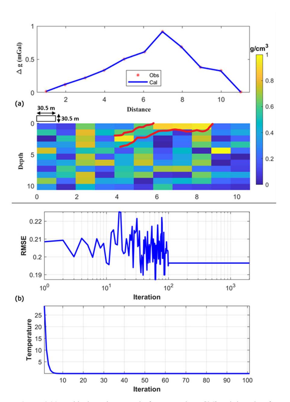
Figure 6 (a) Residual gravity anomaly from Templeton [24] and the subsurface modeling domain. The solid red line depicts the area where the presence of sulphide ore body was identified by Templeton [18] and by Last and Kubik [9] using compact gravity inversion. (b) RMSE variation and temperature decrease with respect to number of iterations.

The final value of the density contrast depends on the RMSE value of the accumulated results of all model parameters, which is a result of the ambiguous nature of gravity modeling. When density values are selected on the above model spaces that produce the smallest RMSE, then the inverted model that still has artifacts can be considered the best model to represent the real model. Certainly, this is an example of the weakness of using vertical and horizontal constraints for targets with a dipping geometry.

The variation of RMSE values as the number of iterations progresses is shown in Figure 6(b). They reach stability after about 100 iterations. This stability reflects the stability of the inverted solution, which also indicates that the global optimum is reached at a slow decrease of temperature, as depicted in Figure 6(b).

4 Conclusions

The application of Very Fast Simulated Annealing (VFSA) inversion to a continuous two-dimensional gravity problem was implemented. The modeling domain was discretized into smaller sub-domains or boxes and a Talwani-based formulation was used to calculate the residual gravity response at the stations on the surface. This attempt may be regarded as a completion of previously reported applications of VFSA for cases of simple and fixed geometries. The VFSA scheme was tested by inverting gravity data generated by simple models. Ten percent of random noise was added to the data before inversion. Due to inherent under-determined nature of the problem and noise in the data, the results showed that insertion of a symmetry axis as a constraint is not adequate to reveal an inverted model that is close enough to the test model. Addition of specific constraints to the problem improves the closeness of the inverted models to the test models, even though it cannot provide an exact fit. Within the scope of this study, VFSA inversion ensures the stability of the solution, which can be attributed to the achievement of a global optimum and robustness against noise at the expense of time computation.

This VFSA scheme was tested also to invert real data measured in a previously published massive sulphide complex. The results more or less show reliable applicability of this scheme for use in two-dimensional gravity interpretation. However, the limitations of this scheme should be borne in mind, particularly regarding artifacts that emerge in the inverted density model.

Acknowledgements

The authors wish to express their gratitude to the Research, Community Empowerment and Innovation Program of Institut Teknologi Bandung (P3MI –

LPPM ITB) 2017 for partially funding this research. They are also deeply indebted to the Modeling & Inversion Laboratory of Physics of Earth and Complex Systems, ITB for facilitating the computational aspects of this research.