
1 Introduction
The flow past a semi infinite flat plate is a well known model in fluid dynamics. Stewarton [1,2] have done significant studies to find out the nature of the flow in the boundary layer. The effect of the magnetic field on flow has large implications in the development of devices such as magnetohydrodynamic generators, MHD pumps, heat exchangers, nuclear reactors, oil exploration, etc. In recent years, substantial analysis has been done in the study of factors that affect MHD boundary layer flow. For instance, a model that includes the effects of radiation and mass transfer on an impulsively started infinite vertical plate was studied in Prasad, et al. [3]. They solved the model using a finite-difference method and observed that the velocity of the flow decreased in the boundary layer when the radiation parameter was increased. Sharidan, et al. [4] have investigated the effects of radiative heat and mass transport on time dependent MHD convective flow through a porous medium past an infinite plate with ramped plate temperature. They obtained analytical solutions for the velocity, temperature and concentration fields by using an integral transform technique and found that increasing the inclination angle and radiation decreases the fluid velocity along the plate. Recently, an analysis of unsteady MHD Eyring-Powell
Received March, 9th, 2017, 1st Revision February 20th, 2019, 2nd Revision April 7th, 2019, Accepted for publication May, 20th, 2019.
Copyright © 2019 Published by ITB Journal Publisher, ISSN: 2337-5760, DOI: 10.5614/j.math.fund.sci.2019.51.3.4
squeezing flow in a stretching channel was studied by Ghadikolaei, et al. [5]. They have also studied [6] the thermal radiation effect on a magneto Casson nanofluid over an inclined porous stretching sheet. They found that the temperature in the system increases with an increase in radiation. Further, considerable interest has been shown by researchers in the effects of heat generation/absorption in moving fluids with convection for heat and mass transfer. Some of these studies are mentioned here. MHD flow of a uniformly presence stretched vertical permeable surface in the generation/absorption was studied by Chamka [7]. Makinde and Mhone [8] analyzed the combined effects of a transverse magnetic field and radiative heat transfer. Recently, a numerical investigation on ethylene glycol-titanium dioxide nano-fluid convective flow has been conducted by Hosseinzadeh, et al. [9]. Further, two important models related to MHD free convective flow past an infinite vertical flat surface have been analyzed by Rajput and Gaurav [10] and Prasad, et al. [11].
Reports on heat transfer and hydrodynamic characteristics of rotating flows have been published by Rajput and Shareef [12], Soong and Ma [13], Soong [14], Greenspan [15], Muthucumaraswamy, et al. [16], and Owen and Rogers [17]. A number of similar models [18-23] that have been studied are mentioned in the reference section.
The model under consideration is solved by the Laplace transform technique. The results are explained using graphs and a table. The table contains data related to skin friction.
2 Mathematical Analysis
Let the X-axis be taken along the plate and Z normal to the plate. The fluid and the plate rotate together as a rigid body with a uniform angular velocity \(\overline{\Omega}\) about the Z-axis. A uniform magnetic field \(B_o\) [Tesla] is applied along the Z-axis. As the plate occupying the plane Z=0 is of infinite extent, all the physical quantities depend only on Z and time \(\tau\) [sec]. Initially, at time \(\tau \leq 0\), the plate and the fluid are at rest, and at a uniform temperature, \(\overline{T}_{\infty}\). At time \(\tau > 0\), the plate starts oscillating in the vertical direction with velocity \(u_o \cos \overline{\omega} \tau\) in its own plane, and the temperature of the plate is raised to \(\overline{T}_p\). The fluid considered is electrically conducting, with a very small Reynolds number, hence the induced magnetic field produced is negligible in comparison to the applied one. Also, due to the conservation of electric charge, the current density along the Z-direction, \(\overline{J}z\), is constant. The plate is assumed to be non-conducting and hence \(\overline{I}z\) is taken as zero. Table 1 is the nomenclature that used in this research.
Table 1 Nomenclature used in this research.
| \(\bar{u}\) primary velocity of the fluid[m/sec] | \(\beta\) volumetric coefficient of thermal |
| \(\bar{v}\) secondary velocity of the fluid [m/sec] | expansion |
| \(\overline{T}\) temperature of the fluid [K] | R radiation parameter |
| \(\alpha\) thermal diffusivity \([m^2/sec]\) | m Hall parameter |
| \(c_p\) specific heat capacity [J/Kg-K] | |
| \(k_{\rho}\) mean absorption coefficient | Non-dimensional constants: |
| \(u_0\) amplitude of initial velocity \([m/sec]\) |
|
| k thermal conductivity \([W/(m \cdot K)]\) | v secondary velocity of the fluid |
| \(\bar{J}_x\) current density along X-axis | \(\theta\) temperature of the fluid |
| \(\bar{J}_{y}\) current density along Y-axis | z space coordinate normal to the plate |
| \(\frac{\check{\bar{K}}}{\bar{K}}\) permeability parameter | \(\omega\) angular frequency of oscillation |
| \(Q_0\) heat source parameter | K permeability parameter |
| \(\overline{\omega}\) angular frequency of oscillation [sec-1] | \(\Omega\) rotation parameter |
| v kinematic viscosity | Q heat source parameter |
| g gravitational aceleration | \(P_r\) Prandtl number |
| \(\sigma\) Stefan-Boltzmann constant [\(Wm^{-2}K^{-4}\)] | M magnetic field parameter |
| \(q_r\) radiative heat flux | \(G_r\) thermal Grashof number |
| \(\rho\) density of the fluid[\(kg/m^3\)] | |
| p women's or me name[ng/m] |
The complete mathematical model is as follows:
\[\frac{\partial \overline{u}}{\partial \tau} - 2\overline{\Omega v} = v \frac{\partial^2 \overline{u}}{\partial Z^2} + g\beta(\overline{T} - \overline{T}_{\infty}) + \frac{B_o}{\rho} \overline{J}_Y - \frac{v}{\overline{K}} \overline{u}, \tag{1}\]
\[\frac{\partial \overline{v}}{\partial \tau} + 2\overline{\Omega u} = v \frac{\partial^2 \overline{v}}{\partial Z^2} - \frac{B_o}{Q} \overline{J}_X - \frac{\mu}{\overline{K}} \overline{v}, \tag{2}\]
\[\frac{\partial \overline{T}}{\partial \tau} = \frac{k}{\rho c_p} \frac{\partial^2 \overline{T}}{\partial Z^2} - \frac{1}{\rho c_p} \frac{\partial q_r}{\partial Z} + \frac{Q_o}{\rho c_p} (\overline{T} - \overline{T}_{\infty}), \tag{3}\] where \[\overline{J}_X = \frac{\sigma B_o(v + m\overline{u})}{1 + m^2}, \overline{J}_Y = \frac{\sigma B_o(m\overline{v} - \overline{u})}{1 + m^2}.\]
The following appropriate boundary conditions are taken:
\[\tau \leq 0: \overrightarrow{u} = 0, \quad \overrightarrow{v} = 0, \quad \overrightarrow{T} = \overrightarrow{T}_{\infty} \quad \forall Z, \tau > 0: \overrightarrow{u} = u_{0} \cos(\overrightarrow{\omega} \tau), \quad \overrightarrow{v} = 0, \quad \overrightarrow{T} = \overrightarrow{T}_{p} \text{ at } Z = 0, \overrightarrow{u} \rightarrow 0, \quad \overrightarrow{v} \rightarrow 0, \quad \overrightarrow{T} \rightarrow \overrightarrow{T}_{\infty} \quad \text{as } Z \rightarrow \infty.\] \[(4)\]
Considering the Rosseland approximation (Brewster [24]), the radiative heat flux \(q_r\) is taken as:
\[q_r = -\frac{4\sigma}{3k_a} \frac{\partial \overline{T}^4}{\partial Z}.\] (5)
If temperature differences in the system are sufficiently small, then, neglecting the higher order terms in the Taylor series expansion of \(\bar{T}^4\) about \(\bar{T}_{\infty}\), we get:
\[\overline{T}^4 \cong 4\overline{T}_{\infty}^3 \overline{T} - 3\overline{T}_{\infty}^4. \tag{6}\]
By using Eq. (5) and Eq. (6), Eq. (3) reduces to:
\[\frac{\partial \overline{T}}{\partial \tau} = \alpha \frac{\partial^2 \overline{T}}{\partial Z^2} + \frac{16\sigma \overline{T}_{\infty}^3}{3k_e \rho C_p} \frac{\partial^2 \overline{T}}{\partial Z^2} + \frac{Q_o}{\rho c_p} (\overline{T} - \overline{T}_{\infty}) \text{ or}\] \[\frac{\partial \overline{T}}{\partial \tau} = \alpha \left( 1 + \frac{4}{3R} \right) \frac{\partial^2 \overline{T}}{\partial Z^2} + \frac{Q_o}{\rho c_p} (\overline{T} - \overline{T}_{\infty})\] where \(R = \frac{k_e k}{4\sigma \overline{T}_{\infty}^3}\). (7)
To make the equations dimensionless, we introduce the following nondimensional quantities:
\[u = \frac{\overline{u}}{u_o}, \quad v = \frac{\overline{v}}{u_o}, \quad t = \frac{u_o^2}{v}\tau, \quad K = \frac{u_o^2}{v^2}\overline{K}, \quad z = \frac{u_o}{v}Z,\] \[\theta = \frac{\overline{T} - \overline{T}_{*}}{\overline{T}_p - \overline{T}_{*}}, \quad Q = \frac{v}{\rho u_o^2}Q_o, \quad P_r = \frac{v}{\alpha}, \quad M^2 = \frac{\sigma B_o^2 v}{\rho u_o^2},\] \[G_r = \frac{g\beta v(\overline{T}_p - \overline{T}_{*})}{u_o^3}, \quad \Omega = \frac{v}{u_o^2}\overline{\Omega}, \quad \omega = \frac{v}{u_o^2}\overline{\omega}.\] \[(8)\]
Eq. (1), Eq. (2), Eq. (7) and Eq. (4) become:
\[\frac{\partial u}{\partial t} - 2\Omega v = \frac{\partial^2 u}{\partial z^2} + \frac{M}{(1+m^2)} (mv - u) + G_r \theta - \frac{u}{K},\tag{9}\]
\[\frac{\partial v}{\partial t} + 2\Omega u = \frac{\partial^2 v}{\partial z^2} - \frac{M}{(1+m^2)} (v + mu) - \frac{v}{K},\tag{10}\]
\[\frac{\partial \theta}{\partial t} = \frac{R_a}{P} \frac{\partial^2 \theta}{\partial z^2} + Q\theta,\tag{11}\]
\[t \le 0: u = 0, \quad v = 0, \quad \theta = 0 \quad \forall z.\] \[t > 0: u = \cos(\omega t), \quad v = 0, \quad \theta = 1 \quad at \quad z = 0.\] \[u \to 0, \quad v \to 0, \quad \theta \to 0 \quad as \quad z \to \infty.\] \[(12)\]
For finding the velocity, we combine Eq. (9) and Eq. (10) and by taking V = u + iv, we get:
\[\frac{\partial V}{\partial t} = \frac{\partial^2 V}{\partial z^2} - b V + G_r \theta, \tag{13}\]
The boundary conditions in Eq. (12) are reduced to:
\[t \le 0: V = 0, \ \theta = 0 \quad \forall z.\] \[t > 0: V = cos(\omega t), \quad \theta = 1 \quad at \quad z = 0.\] \[V \to 0, \quad \theta \to 0 \quad as \ z \to \infty.\] \[(14)\]
The model given by partial differential Eq. (11) to Eq. (13) with boundary conditions in Eq. (14) is solved by the Laplace transform technique. The solution obtained is as follows:
\[\begin{split} \theta(z,t) &= \frac{1}{2} \left\{ e^{-ia_9 z} Erf \left( i\sqrt{Qt} - a_7 \frac{z}{\sqrt{t}} \right) - e^{ia_9 z} Erf \left( i\sqrt{Qt} + a_7 \frac{z}{\sqrt{t}} \right) \right\} + Cosh(a_9 z) \\ V(z,t) &= -\frac{Cos\omega t}{2} \left\{ -2Cosh(a_1 z) + \frac{1}{2} e^{-a_1 z} Erf \left( \frac{z}{2\sqrt{t}} - a_1 \sqrt{t} \right) + \frac{1}{2} e^{a_1 z} Erf \left( \frac{z}{2\sqrt{t}} + a_1 \sqrt{t} \right) \right\} \\ &+ a_5 \left[ -e^{-a_2 z} Erf \left( a_2 \sqrt{t} - \frac{z}{2\sqrt{t}} \right) - e^{a_2 z} Erf \left( a_2 \sqrt{t} + \frac{z}{2\sqrt{t}} \right) + 2Cosh(a_9 z) \right] \\ &+ a_5 \left[ e^{-ia_9 z} Erf \left( ia_6 \sqrt{t} - a_7 \frac{z}{\sqrt{t}} \right) - e^{ia_9 z} Erf \left( ia_6 \sqrt{t} + a_7 \frac{z}{\sqrt{t}} \right) + 2Sinh(a_2 z) \right] \\ &+ a_5 e^{Bt} \left[ e^{-a_3 z} Erf \left( a_3 \sqrt{t} - \frac{z}{2\sqrt{t}} \right) - e^{a_3 z} Erf \left( a_3 \sqrt{t} + \frac{z}{2\sqrt{t}} \right) + 2Cosh(a_3 z) \right] \\ &+ a_5 e^{Bt} \left[ e^{-a_8 z} Erf \left( a_4 \sqrt{t} - a_7 \frac{z}{\sqrt{t}} \right) + e^{a_8 z} Erf \left( a_4 \sqrt{t} + a_7 \frac{z}{\sqrt{t}} \right) - 2Cosh(a_8 z) \right] \end{split}\]
3 Skin Friction and Nusselt Number
The non-dimensional skin-friction components in the primary \((\tau_1)\) and secondary \((\tau_2)\) directions are obtained as follows:
\[\tau_1 + i\tau_2 = -\frac{\partial \mathbf{V}}{\partial z}\Big|_{z=0}\] and the expression for the dimensionless Nusselt number is given as:
\[Nu = \frac{\sqrt{a}e^{Qt}}{\sqrt{\pi t}} - \sqrt{aQ} \operatorname{erf}\left(i\sqrt{Qt}\right),\] where
\[\begin{split} b &= \frac{M^2 i}{m+i} + 2i\Omega + \frac{i}{K}, \ R_a = 1 + \frac{4}{3R}, \ a = \frac{P_r}{R_a}, \ A = \frac{G_r}{a-1}, \ B = \frac{b+aQ}{a-1}, \\ a_1 &= \sqrt{(b-i\omega)}, \ a_2 = \sqrt{b}, \ a_3 = \sqrt{(b+B)}, \ a_4 = \sqrt{(B-Q)}, \ a_5 = \frac{A}{2B}, \\ a_6 &= \sqrt{Q}, \ a_7 = \sqrt{\frac{a}{4}}, \ a_8 = \sqrt{a(B-Q)}, \ a_9 = \sqrt{aQ}. \end{split}\]
4 Results and Discussion
From Figure 1 it can be seen that increasing the value of K, the magnitude of the primary and the secondary velocity increases. This is because an increase in K implies a decrease in the resistance of the porous medium. Hence the momentum boundary layer thickness increases with K.
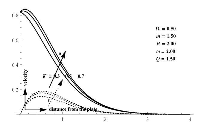
Figure 1 Figure 1. Variation in velocity with K.
The heat source effect on the velocity distribution is shown in Figure 2. Here it is observed that both components of the velocity are accelerated by heat source parameter Q. Hence the effects of the radiation parameter and the heat source parameter on the fluid flow are opposite.
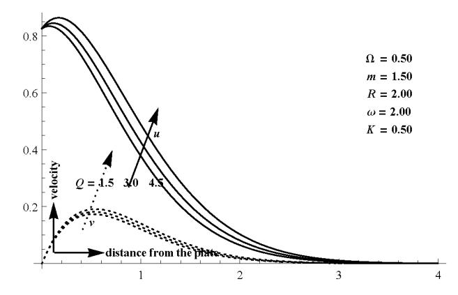
Figure 2 Variation in velocity with Q.
Figure 3 shows the influence of the Hall current on u and v. It can be seen that u increases rapidly near the surface of the plate, whereas v decreases throughout the boundary layer region along with the increasing parameter 'm'. This shows that the Hall current tends to accelerate u in the region near the surface of the plate, whereas it tends to slow down v throughout the boundary layer region. This may be attributed to the fact that the value of the term 1/ሺ1 ଶሻ is very small for large values of 'm'; hence a large 'm' diminishes the resistive effect of the applied magnetic field.
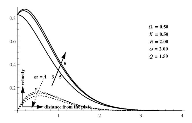
Figure 3 Variation in velocity with m.
Figure 4 shows the effect of R on both components of the velocity. Here it is observed that it slows down the flow. This is because when R increases, the temperature of the system decreases and as a result the fluid flow becomes slower.
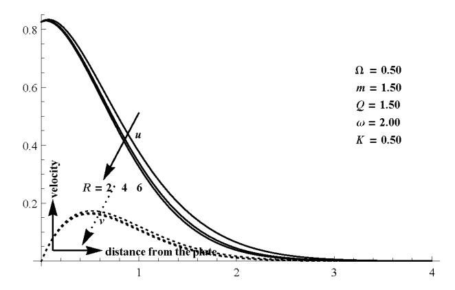
Figure 4 Variation in velocity with R.
The effect of rotation on the flow behavior is shown in Figure 5. It is observed that when Ω increases, u decreases throughout the boundary layer region, whereas v increases continuously near the surface of the plate. This implies that the rotation tends to accelerate v, whereas it slows down u in the boundary layer region.
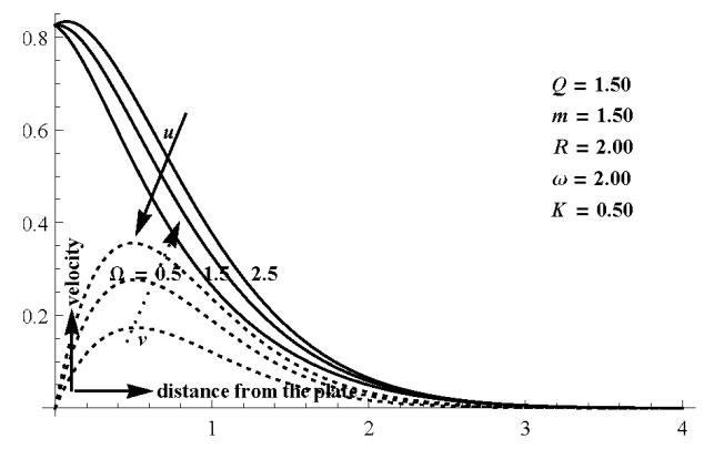
Figure 5 Variation in velocity with Ω.
As the oscillation increases, the primary velocity decreases rapidly near the plate and in the region away from the plate, while v decreases throughout the boundary layer (Figure 6).
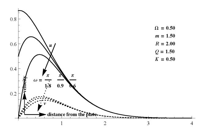
Figure 6 Variation in velocity with ω.
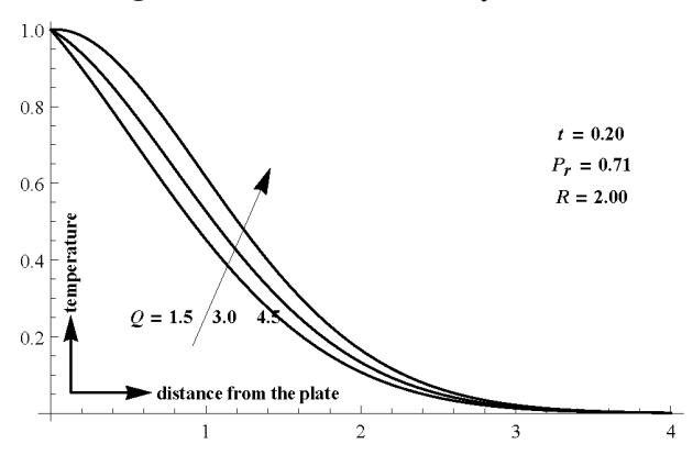
Figure 7 Variation in temperature with Q.
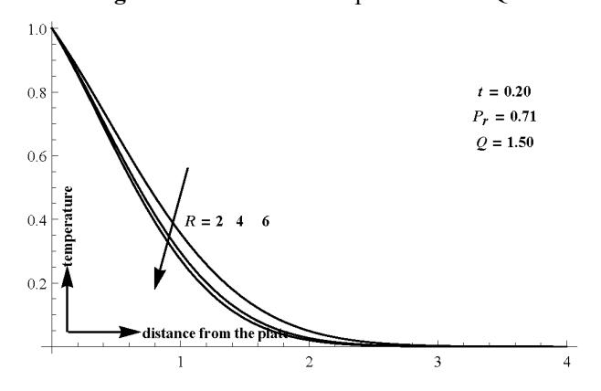
Figure 8 Variation in temperature with R.
The temperature profiles for different values of R and Q and for constant Pr at time t = 0.2 are shown in Figures 7 and 8. In Figure 8, it can be seen that the temperature of the fluid is inversely proportional to the value of radiation
parameter R. Thus the increase in R reduces the temperature in the system. And hence the thermal boundary layer thickness decreases with R. Meanwhile, Figure 7 shows that the temperature in the system increases with increasing Q. The effects of various parameters on the skin-friction at the surface of the plate are shown in Table 2.
| Table 2 Skin interior (at t | (at t | 0.1). | ||||||
|---|---|---|---|---|---|---|---|---|
| m | K | Q | R | Ω | ω | M | \(\tau_1\) | \(-\tau_2\) |
| 1.0 | 0.5 | 1.5 | 2 | 0.5 | \(\pi/0.6\) | 2 | 0.776 | 0.490 |
| 2.0 | 0.5 | 1.5 | 2 | 0.5 | \(^{\pi}/_{0.6}\) | 2 | 0.571 | 0.442 |
| 3.0 | 0.5 | 1.5 | 2 | 0.5 | \(^{\pi}/_{0.6}\) | 2 | 0.497 | 0.380 |
| 1.5 | 0.3 | 1.5 | 2 | 0.5 | \(^{\pi}/_{0.6}\) | 2 | 0.865 | 0.457 |
| 1.5 | 0.6 | 1.5 | 2 | 0.5 | \(^{\pi}/_{0.6}\) | 2 | 0.591 | 0.482 |
| 1.5 | 0.5 | 3.0 | 2 | 0.5 | \(\frac{\pi}{0.6}\) | 2 | 0.626 | 0.478 |
| 1.5 | 0.5 | 4.5 | 2 | 0.5 | \(^{\pi}/_{0.6}\) | 2 | 0.603 | 0.480 |
| 1.5 | 0.5 | 1.5 | 2 | 0.5 | \(^{\pi}/_{0.6}\) | 2 | 0.647 | 0.477 |
| 1.5 | 0.5 | 1.5 | 4 | 0.5 | \(^{\pi}/_{0.6}\) | 2 | 0.689 | 0.473 |
| 1.5 | 0.5 | 1.5 | 6 | 0.5 | \(^{\pi}/_{0.6}\) | 2 | 0.705 | 0.471 |
| 1.5 | 0.5 | 1.5 | 2 | 1.5 | \(^{\pi}/_{0.6}\) | 2 | 0.690 | 0.808 |
| 1.5 | 0.5 | 1.5 | 2 | 2.5 | \(^{\pi}/_{0.6}\) | 2 | 0.753 | 1.134 |
| 1.5 | 0.5 | 1.5 | 2 | 0.5 | \(\frac{\pi}{0.6}\) | 2 | 0.647 | 0.477 |
| 1.5 | 0.5 | 1.5 | 2 | 0.5 | \(^{\pi}/_{0.3}\) | 2 | -1.132 | 0.380 |
| 1.5 | 0.5 | 1.5 | 2 | 0.5 | \(^{\pi}/_{0.2}\) | 2 | -3.373 | 0.240 |
| 1.5 | 0.5 | 1.5 | 2 | 0.5 | \(^{\pi}/_{0.6}\) | 4 | 1.365 | 1.229 |
| 1.5 | 0.5 | 1.5 | 2 | 0.5 | \(\pi/_{0.6}\) | 6 | 2.516 | 2.076 |
Table 2 Skin friction (at t = 0.1).
It can be seen from Table 2 that the value of \(\tau_1\) increases when the values of M, \(\Omega\), R are increased (keeping other parameters fixed); but if the values of m, Q, \(\omega\) and K are increased, the value of \(\tau_1\) decreases. Also, it is observed that the magnitude of \(\tau_2\) increases with M, \(\Omega\), Q and K; and it decreases when m, R and \(\omega\) are increased.
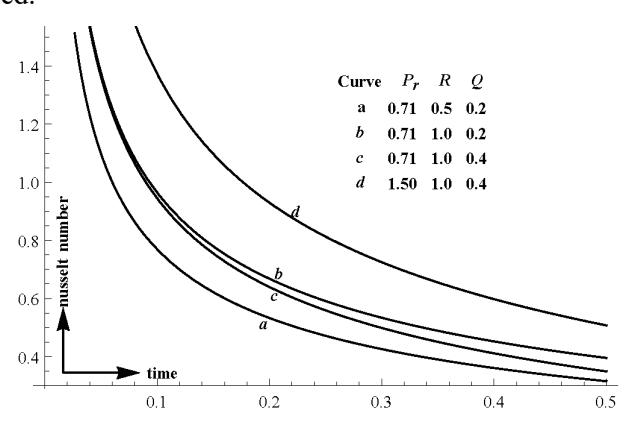
Figure 9 Variation in Nusselt number with time.
The Nusselt number is plotted against time in Figure 9. Here it is observed that initially the number achieves its maximum value at the plate and then decreases continuously as time increases. Also, it can be seen that the Nusselt number decreases with an increase of the heat source parameter and increases with an increase of R or Pr.
5 Conclusion
In this study, it was observed that the Hall current speeds up the primary flow whereas it slows down the secondary flow. The temperature and velocity decrease in the boundary layer with an increase of the radiation parameter. Further, it was noticed that both components of the shear stress increase with a rise of the radiation parameter, and decrease with a rise in the heat source parameter. Also, rotation slows down the primary flow, whereas it speeds up the secondary flow. The outcomes obtained have large implications in studies related to the structure of rotating magnetic stars, solar physics, geophysics and the solar cycle.