
1 Introduction
Software is an integral part of all activities performed on digital platforms, giving it an influence on each and every sector of modern society. The applicability of software has led to enormous growth in the day-to-day workings of business processes [1]. This makes it critical to have software that offers consistent performance and at the same provides highly reliable execution. Ample of cases exist where software was not able to deliver the task assigned, leading to serious damage [2]. Seeing the high dependence of mankind on software and its functionality, it is the foremost responsibility of software developers to create software that is optimally effective and efficient. Thus, testers are hired whose primary task it is to debug the software and make it bugfree before it is provided to end-users. The testing team will try to fix any flaws in order to enhance the quality of the software. Reliability, which is the probability of the failure-free operation of a product for a specific period of time under predefined conditions, is an important aspect of quality [1,3]. Software firms acknowledge the importance of testing their products in the operational phase and provide regular upgrades of their software products in order to maintain their competitive position. Software up-gradation is a survival strategy for firms that helps in maintaining and increasing market share by providing advanced versions with enhanced functionality to users [4]. To a certain extent, publishing several versions is beneficial for firms but under certain circumstances increasing a piece of code may result in the introduction of new faults making the software prone to failure. Firms should focus on adapting techniques capable of identifying and removing a maximum number of faults. It is evident that all potential faults cannot be removed in one go, thus leftover bugs from previous versions can result in software failure. Therefore, getting a clear picture of error removal should be a main priority for software developers [5].
Multi up-gradation cannot be discussed without discussing the release-time problem. The optimal time to release software is an other important concern for software developers, as releasing prematurely will degrade the quality and releasing too late impacts market entry, the cost of software testing and poses many other challenges as well. In the literature, several attempts have been made to formulate and compute the optimal time for launching software based on goals set by management [1]. This can be minimization of costs and other resources, or maximization of reliability, failure intensity and market share subject to various sets of constraints. These sets of constraints have been formulated both under crisp and fuzzy environments. The present study focused on the fuzzy release time decision (FRTD) problem due to its capability of modeling qualitative information of decision-makers and to directly work on fuzzy information [6].
A generic model is proposed to determine bugs that have been removed in each release based on the impact of leftover bugs from the previous release and faults generated as a result of up-gradation. Moreover, a fuzzy release time decision based optimization analysis was performed to determine the release time of software under the influence of the attributes cost and reliability.
This paper is organized as follows. Section 2 presents the background and an overview of the literature on software reliability growth modeling and the fuzzy release time decision problem. The generalized modeling framework for determining faults in respective software releases is discussed in Section 3. Cost modelling is discussed in Section 4.The optimal launch time problem is discussed in Section 5. Validation and a numerical illustration are presented in Sections 6 and 7. Lastly, the conclusion is given in Section 8.
2 Background and Literature Review
A large amount of progress has been made in the study of multi up-gradation. The most basic approach is to compute the reliability of a software product
based on the effect of leftover faults from all of its preceding releases [7,8]. It was soon realized that this approach is not very effective and the influence on the reliability of the software is not very significant [9]. Thus, practitioners started taking into account only the impact of the previous version on the reliability of the present release. Another observation that researchers have made was that the testing team is not always able to remove all faults completely, which can lead to an imperfect debugging environment when only considering faults from the previous release, as modeled by Aggarwal, et al. [10]. Some researchers have studied the concept of stochasticity in multi upgradation [5]. Several experts have analyzed the debugging environment and uncertainty to study the severity of faults and the distribution environment to simulate market scenarios [10,11]. The issues encountered in both the testing and the operational phase were given equal weight [3,12].
The study by Singh, et al. [13] considered the effect of a Weibull type testing effort function (TEF) on the detection of faults in multiple versions of a software application. They further explain that TEF for each release follows an exponential and S-shaped curve. Kapur, et al. [14] developed an optimal cost model to find out the testing stop time for each release. They considered the accumulation of various costs incurred during the testing phase of new releases and the removal of leftover faults in the operational phase of the ongoing version and in the testing phase of the upcoming release. Singh, et al. [15] have proposed a unified approach to model successive releases of software under the influence of imperfect debugging. Numerous studies exist in the literature describing the fault removal phenomenon for multi up-gradation software versions and the associated cost analysis.
Several release-time policies have been proposed in the field of software reliability. The first ever release policy was given by Goel and Okumoto [16] to determine release time based on unconstrained cost minimization and reliability maximization as two separate sets of problems. Later, several release policies have been presented with different sets of optimization problems, for example: Yamada and Osaki [17] considered the joint impact of cost and reliability on the determination of optimal time to introduce the software on the market. Yun and Bai [18] focused on software with a random lifecycle and cost-based modeling for the determination of the optimal release time. Other researchers who have worked under same umbrella of cost analysis are: Huang [19]; Huang and Lyu [20]; Pham and Zhang [21]; Ramik [22]; Rommelfanger [23]; Tang and Wang [24];Ukimoto and Dohi [25] Xie and Yang [26]; and Yang, et al. [27].
All of the aforementioned scholars have worked on finding the optimal release time for a single software version. Very few attempts have been made to model and find the optimal software release time for multi up-graded software
systems. Something similar has been done by Kapur, et al. [14], who applied the concept of multi-attribute utility theory. However, these attempts were all done under a crisp environment. The field of cost optimization also deals with cases involving vagueness or fuzziness. This is an appealing topic in the field of software reliability, based on which a number of FRTD problems have been proposed. Models defined by utilizing fuzzy theory represent the conversion of subjective information and can help in incorporating vagueness in traditional crisp optimization problems. Kapur, et al. [28] formulated a fuzzy environment based on the cost minimization problem under constraint of failure intensity. Working from a similar starting-point, Jha, et al. [29] proposed a discrete SRGM-based FRTD problem by considering the cost and reliability objectives subject to budgetary constraints under a crisp scenario. Later, Jha, et al. [30] extended their work on the FRTD problem under the concept of imperfect debugging and an error generation software reliability growth model. Kumar, et al. [6] proposed an FRTD problem based on testing cost under the impact of warranty period. Recently, Kumar and Gupta [31] looked at an FRTD problem incorporating the effect of learning functions for fault detection and correction. However, none of these efforts were related to multi-upgraded software systems. As discussed above, and as per our available knowledge, this is the first attempt to model multi up-gradation under a fuzzy environment.
3 Modeling Methodology
The notation used in this paper is the following:
i : number of versions (i = 1,2,3,4) \(m_i(t)\) : mean value function for fault removal \(a_i\) : total count of faults present in the software
\(b_i\): rate of fault debugging \(\beta_i\): learning parameter
Supposing the case of multi-upgraded software and assuming that the first version of the software was initially launched at time point \(t_1 = 0\) and the launch time of the succeeding \(i^{th}\) release will be \(t_i\). The actual count of faults debugged in the \(i^{th}\) release of the software can be obtained as follows:
\[m_i(t) = Y_i(t)F_i(t) \tag{1}\]
Eq. (1) tries to elucidate the fraction \(F_i(t)\) of the total number of faults \(Y_i(t)\) that can be debugged from the total fault count of any particular release. Also note that \(F_i(t)\) represents the fraction of faults in the \(i^{th}\) version of the software that will be debugged in the \(i^{th}\) release of the software until the time period t', whereas t' represents the number of bugs in the t' release, consisting of both the faults generated due to the addition of new features and bugs remaining from the preceding release. The fraction of faults has the following mathematical form:
\[F_{i}(t) = \begin{cases} 0 & t \le t_{i} \\ F_{i}(t - t_{i}) & t_{i} < t < t_{i+2} \\ 1 & t \ge t_{i+2} \end{cases}\] (2)
In Eq. (2), it is important to note that if \(t < t_i\) it means that the \(i^{th}\) release has not been tested yet, while if \(t = t_i\) it means that the software has been given to testing team to begin debugging. Thus, in both cases the count of bugs discovered will be zero. If \(t > t_{i+2}\) then the fraction of bugs discovered will be exactly one. Further, if \(t_i < t < t_{i+2}\) then there is a positive fraction of faults being debugged for the \(i^{th}\) release at time point t'.
The \(Y_i(t)\) represents the number of bugs generated in the \(i^{th}\) release of the software with addition of the leftover faults from the \((i-1)^{th}\) release. Thus (for i > 1), \(Y_i(t)\) can be defined as:
\[Y_{i}(t) = Y_{i-1} \left[ 1 - F_{i-1}(t_{i}) \right] + a_{i}\] (3)
where \(a_1\) represents the faults in the first release (for i = 1 we define \(Y_1(t) = a_1\)) and thereafter the faults of the succeeding releases are denoted by \(a_1, i > 1\). The present proposal focuses on the case of four releases of the software.
Primary Release: Substituting i = 1 in Eqs. (1), (2) and (3) yields:
\[m_1(t) = Y_1(t)F_1(t) \tag{4}\] where \(Y_1(t) = a_1\) and \(F_1(t) = F_1(t - t_1)\)
First Upgraded Version: Substituting i = 2 in Eqs. (1), (2) and (3), the fault removal process for the first upgraded version can be given as follows:
\[m_2(t) = Y_2(t)F_2(t) \tag{5}\] where \[Y_2(t) = a_1 [1 - F_1(t_2 - t_1)] + a_2\] and \(F_2(t) = F_2(t - t_2)\)
By substituting we get:
\[m_{2}(t) = \left[ a_{2} + a_{1} \cdot (1 - F_{1}(t_{2} - t_{1})) \right] F_{2}(t - t_{2})\] (6)
Second Upgraded Version: By considering i = 3 in Eqs. (1), (2) and (3), we have:
\[m_3(t) = Y_3(t)F_3(t)\] (7)
where \[Y_3(t) = a_2[1 - F_2(t_3)] + a_3\] and \(F_3(t) = F_3(t - t_3)\)
By substituting we get:
\[m_3(t) = \left[ a_3 + a_2 \left( 1 - F_2 \left( t_3 - t_2 \right) \right) \right] F_3(t - t_3) \tag{8}\]
Similarly, the results for the third upgraded version can be obtained:
\[m_4(t) = \left[ a_4 + a_3 \left( 1 - F_3 \left( t_4 \right) \right) \right] F_4 \left( t - t_4 \right) \tag{9}\]
4 Cost-Modeling for Multi Upgraded Software
The formulation of the optimal time of successive software releases determined by an optimization model is based on the objectives set by management. Firstly, management would move in a direction where there is minimum aggregate cost of debugging during the testing and the operational phase. Secondly, they may set the reliability level that is to be attained until the release time of the software on the market.
Release I: The general cost model distinguishes costs in three phases. The testing phase per unit cost of testing; the testing phase cost of debugging; and the operational phase cost of debugging can be given as:
\[C_{1}(t) = C_{\text{per unit testing cost}} + C_{\text{debugging cost in testing phase}}\] \[+ C_{\text{debugging cost in operational phase}}\] \[= C_{10} t^{\gamma} + C_{11} . a_{1} . F_{1}(t) + C_{12} . a_{1} . (1 - F_{1}(t))\] \[(10)\]
Release II: The expenditure incurred for a new release comprises cost of testing of upcoming version, cost of debugging during the operational phase and cost of elimination of passed-on bugs from the prior version during both the testing and the operational phase of the present release.
\[C_{2}(t) = C_{\text{per unit testing cost}} + C_{\text{debugging cost in testing phase}}\] \[+ C_{\text{debugging cost of remaining faults from previous release}}\] \[+ C_{\text{debugging cost in operational phase}}\] \[(11)\]
\[\begin{split} &= C_{20}.t^{\gamma} + C_{21}.a_2.F_2\left(t - t_1\right) + C_{22}.a_1.\left(1 - F_1\left(t_1\right)\right).F_2\left(t - t_1\right) \\ &+ C_{23}.\left(\begin{bmatrix} a_2 + a_1.\left(1 - F_1\left(t_1\right)\right)\end{bmatrix}\right); \quad t_1 \leq t \end{split}\]
Release III: It is assumed that the remaining faults in Release II will either be removed during the testing phase or during the operational phase of Release III. Thus, the total expected cost to debug the faults can be modeled as follows:
\[C_{3}(t) = C_{30} t^{\gamma} + C_{31} \cdot a_{3} \cdot F_{3}(t - t_{2}) + C_{32} \cdot a_{2} \cdot (1 - F_{2}(t_{2})) \cdot F_{3}(t - t_{2})\] \[+ C_{33} \cdot \left[ \left[ a_{3} + a_{2} \cdot (1 - F_{2}(t_{2})) \right] \right]; \qquad t_{2} \leq t\] \[(12)\] where \(C_{30}\) represents the testing cost per unit incurred in Release III; \(C_{31}\) denotes the cost due to debugging done in the testing phase; \(C_{32}\) represents the cost incurred in dealing with the leftover faults of the previous release; \(C_{33}\) is the cost incurred for the debugging done in the operational phase.
Similarly, the total cost linked with Release IV can be given as follows:
\[C_{4}(t) = C_{40} \cdot t^{\gamma} + C_{41} \cdot a_{4} \cdot F_{4}(t - t_{3}) + C_{42} \cdot a_{3} \cdot (1 - F_{3}(t_{3})) \cdot F_{4}(t - t_{3}) + C_{43} \cdot \left[ \left[ a_{4} + a_{3} \cdot (1 - F_{3}(t_{3})) \right] \right]; \qquad t_{3} \le t\] \[(13)\] where \(C_{40}\) is the testing cost per unit incurred in Release IV; \(C_{41}\) is the cost due to debugging done during the testing phase of the release; \(C_{42}\) denotes the cost of dealing with the leftover faults of Release III; \(C_{43}\) is the cost incurred for the debugging done in the operational phase of the fourth release.
5 Optimal Release-Time Problem
All the above mentioned sets of costs, Eq. (10) to (13), are used in order to determine the release time of the respective releases of the software, for which the decision-making problem can be defined as follows:
Min \[C_i(t)\]
Subject to \(R_i(x|t) \tilde{\geq} R_{0i}\); \(i = 1, 2, 3, 4\) (14)
The solution to Eq. (14) can be obtained by using the fuzzy optimization approach given by Zimmermann [32]. The first step is to convert the problem by adding a fuzzifier in the objective function as a limit to the constraint [33]. Thus, the restated problem may have the following structure:
Find \[t\]
Subject to \(C_i(t) \tilde{\leq} C_{0i}\) (15)
\(R_i(x|t) \tilde{\geq} R_{0i}; t \geq 0; i = 1,2,3,4\)
Further, the membership functions \(\mu_{ij}(t)\); i = 1, 2, 3, 4 and j = 1, 2 for each of the fuzzy inequalities can be defined as:
\[\mu_{i1}(t) = \begin{cases} 1 & ; C_i(t) \le C_{0i} \\ \frac{C_i^* - C_i(t)}{C_i^* - C_{0i}} & ; C_{0i} < C_i(t) \le C_i^* \\ 0 & ; C_i(t) > C_i^* \end{cases}\] (16)
\[\mu_{i2}(t) = \begin{cases} 1 & ; R_i(x|t) \ge R_{0i} \\ \frac{R_i(x|t) - R_i^*}{R_{0i} - R_i^*} & ; R_i^* \le R_i(x|t) < R_{0i} \\ 0 & ; R_i(x|t) < R_i^* \end{cases}\] (17)
In Eq. (16), \(C_{0i}\) and \(C_i^*\) represent the available budget and the maximum tolerance value for the budget. In Eq. (17), \(R_{0i}\) and \(R_i^*\) represent the maximum level of reliability to be maintained and the minimum tolerance value of reliability. Subsequently, the principle of Bellman and Zadeh [34] is used to recognize the fuzzy decision by solving the fuzzy set of inequalities for the corresponding problem. The resultant crisp optimization problem can be given as follows:
Maximize \[\alpha_i\]
Subject to \(\mu_{ij}(t) \ge \alpha_i\) \(i = 1, 2, 3, 4; j = 1, 2;\) (18)
\(\alpha_i \ge 0, t \ge 0\)
After solving Eq. (18) and incorporating the parameter values, we can calculate the optimal time to release for each particular version of the software on the market.
6 Data Analysis
For the purpose of estimation, fault removal process \(F_i(t)\) was assumed to follow Yamada logistic pattern [1], which can be given as follows:
\[F_{i}(t) = \frac{1 - (1 + b_{i}(t - t_{i})) \cdot e^{-b_{i}(t - t_{i})}}{1 + \beta_{i} \cdot e^{-b_{i}(t - t_{i})}}; i = 1, 2, 3, 4\] (19)
The proposed model was analyzed on four different releases of the data sets given by Sun [35] using the SAS software package [36]. The estimated values of the parameters of the proposed models were computed using the non-linear least square method, as shown in Table 1 while the comparison criteria are shown in Table 2. The estimated values of the parameters were quite close to the actual values, which indicates the prediction capacity of the model. Goodness of fit curves are represented in Figure 1.
Table 1 Parameter estimates for four releases.
| Parameters | Release 1 | Release 2 | Release 3 | Release 4 |
|---|---|---|---|---|
| а | 604.5 | 443.449 | 362.221 | 440.489 |
| b | 0.434 | 0.449 | 0.845 | 0.591 |
| β | 5.133 | 0.541 | 21.319 | 5.928 |
Table 2 Comparison criteria for four releases.
| Criterion | Release 1 | Release 2 | Release 3 | Release 4 |
|---|---|---|---|---|
| SSE | 1220.2 | 1846.8 | 1565.5 | 2075.6 |
| MSE | 93.865 | 142.1 | 195.7 | 259.5 |
| Root MSE | 9.688 | 11.919 | 13.989 | 16.107 |
| \(R^2\) | 0.998 | 0.993 | 0.991 | 0.992 |
| AIC | 119.708 | 118.818 | 79.559 | 90.018 |
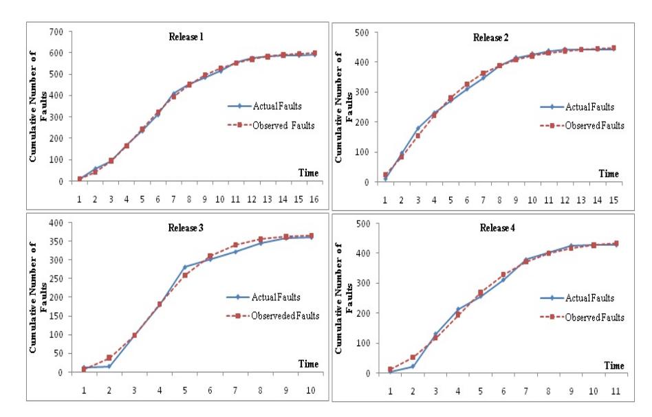
Figure 1 Goodness of fit curves for four releases.
7 Numerical Illustration
For application of the proposed release-time policy, the parameters as obtained in Table 1 were used.
Release I: Considering the parameters as \(a_1 = 604.5, b_1 = 0.434\) and \(\beta_1 = 5.133\). Let us assume that the cost parameters are \(C_{10} = \$18\), \(C_{11} = \$21\), and \(C_{12} = \$48\). Also, the operational mission time is assumed as x = 1 CPU hour and learning parameter y = 0.85. Further, it was assumed that the total budget available for testing purpose \(C_0 = \$12,110\) and the reliability requirement of \(R_{01} = 0.95\), with tolerance on cost and reliability \(C^* = \$15,000\) and \(R_1^* = 0.75\) (these assumed values may vary as they are set by management based on past experience). The MVF for failure and the reliability function can be given as follows:
\[m(t) = \frac{604.5(1 - (1 + 0.434 * t)e^{-0.434 * t})}{(1 + 5.133e^{-0.434 * t})} \text{ and } R(x|t) = e^{-(m(t+1) - m(t))}.\]
Correspondingly the membership function pertaining to the fuzzy cost and the reliability constraint can be defined as:
\[\text{[rumus tidak dapat ditampilkan dengan baik — lihat PDF asli]}\] where \(12110 < C(t) \le 15000\)
\[\mu_2(t) = \frac{e^{-(m(t+1)-m(t))} - 0.75}{0.95 - 0.75}\] where \[0.75 \le e^{-(m(t+1)-m(t))} < 0.95\]
On plotting both membership functions, an intersection point is obtained that describes the optimal introduction time of software release, which can also be computed by solving the crisp optimization problem using an optimization solver such as LINGO [37].
Maximize \[\alpha\] Subject to \[\begin{pmatrix} 18*t^{0.85} \\ + \left(21*604.5*\left(1-\left(1+0.434*t\right)e^{-0.434*t}\right) \\ + \left(1+5.133e^{-0.434*t}\right) \end{pmatrix}\] \[\mu_{1}(T) = \frac{e^{-(m(t+1)-m(t))} - 0.75}{0.95 - 0.75} \ge \alpha\] \[\alpha \ge 0, \quad \alpha \le 1, \quad t \ge 0\]
Solving the above problem, we obtained optimal release time \(t^* = 23.64\) and \(\alpha^* = 0.7028\).
Release II: Proceeding in the same manner as for Release I, the parameter values for the second release were: \(a_2 = 443.44\), \(b_2 = 0.434\) and \(\beta_2 = 0.541\). Assuming the cost parameters to be \(C_{20} = \$25\), \(C_{21} = \$30\), \(C_{22} = \$45\), and \(C_{23} = \$48\). The operational mission time and value for the learning parameter were kept the same. Further, it was assumed that the total budget available for the purpose of testing \(C_0 = \$10,000\) and the reliability requirement \(R_{02} = 0.95\), with tolerance on cost and reliability \(C^* = \$15,000\) and \(R_2^* = 0.75\). Solving the problem, the optimal time to release the software \(t^* = 19.56\) with \(\alpha^* = 0.2058\).
Release III: Proceeding in the same manner as for Release I, the parameter values for the second upgraded version (the third release) were: \(a_3 = 362.221\), \(b_3 = 0.845\) and \(\beta_3 = 21.319\). Assuming the cost parameters to be \(C_{30} = \$15\), \(C_{31} = \$19\), \(C_{32} = \$30\), and \(C_{33} = \$65\). The operational mission time and value for learning parameter were kept the same. Further, it was assumed that the total budget available for the purpose of testing \(C_0 = \$1,500\) and the reliability requirement \(R_{03} = 0.95\), with tolerance on cost and reliability \(C^* = \$10,000\)
and \(R_3^* = 0.75\). Solving the problem, the optimal time to release the software \(t^* = 12.86\) with \(\alpha^* = 0.3346\).
Release IV: Following the same procedure as for Release I, the parameter values for the third upgraded version (the fourth release) were: \(a_4 = 440.48\), \(b_4 = 0.591\) and \(\beta_4 = 5.928\). Assuming the cost parameters to be \(C_{40} = \$15\), \(C_{41} = \$26\), \(C_{42} = \$38\), and \(C_{43} = \$48\). The operational mission time and value for the learning parameter were kept the same. Further, it was assumed that the total budget available for purpose of testing \(C^* = \$11,000\) and the reliability requirement \(R_{04} = 0.95\), with tolerance on cost and reliability \(C^* = \$15,000\) and \(R_4^* = 0.75\). Solving the problem, the optimal time to release the software \(t^* = 17.77\) with \(\alpha^* = 0.8198\).
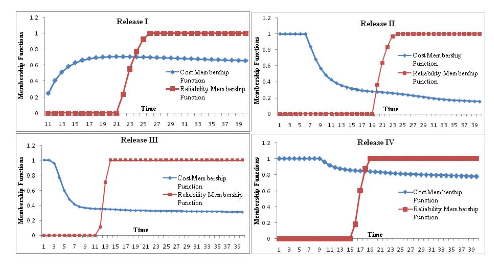
Figure 2 Membership function of cost and reliability for four releases.
Both membership functions corresponding to cost and reliability were plotted for all releases, as shown in Figure 2. There is a clear intersection point of both curves, indicating the optimal launch time for the software. The obtained results corresponding to each release of the software can be summarized in tabular form as given in Table 3.
| Table 3 | Optimal | release | time | for al | l rel | leases. |
|---|
| Releases | \(t^*\) | \(\boldsymbol{\alpha}^*\) | Actual release time |
|---|---|---|---|
| Release-I | 23.64 | 0.7028 | 16 |
| Release-II | 19.56 | 0.2058 | 15 |
| Release-III | 12.86 | 0.3346 | 10 |
| Release-IV | 17.77 | 0.8198 | 11 |
From Table 3 it can be clearly seen that each software release was subjected to under-testing. Thus it is wise to assume that for achieving the threshold value of reliability, the software should be tested for a longer duration.
8 Conclusion
To make the software bug free and enhance its operational capability, firms keep testing and trying to fix them by issuing consecutive upgrades. With this in mind, an alternative mathematical framework was presented in this paper that can capture the faults generated due to addition of certain novel features and leftover faults from its immediately preceding release. The set of proposed models was analyzed on real-life data sets of four different releases. Further, fuzzy release time problems were constructed for the four versions of the software and the optimal time to launch of each version was computed.
Acknowledgments
The work reported in this paper was supported by grants to the first author from the Department of Science and Technology, India through DST PURSE PHASE II scheme, India; and to the second author from the Rajiv Gandhi National Fellowship from University Grants Commission, New Delhi, India and fourth author would like to be thankful to National Research Foundation (South Africa) for the financial support.