
1 Introduction
Diarrhoeal diseases are a significant cause of childhood mortality and morbidity worldwide, accounting for around 525,000 deaths annually in children under five [1]. Diarrhoeal diseases usually occur from contaminated food and water sources. There are many causes of diarrhoeal infections such as viruses, bacteria, or parasites. Rotavirus is one of several viruses that are the most significant causes of acute diarrhoea among children worldwide [2]. Every infant is predicted to have at least one episode with rotavirus before the age of five years, with severe infections occurring between the age of 4 to 23 months [3]. Approximately 215,000 deaths of children are recorded annually due to rotavirus diarrhea, with 56% of the deaths ensuing in Sub-Saharan Africa [4]. Based on VP6 antigen, rotavirus is grouped into at least eight different species, named A to H [5]. Species A is the primary cause of rotavirus disease in humans (acute gastroenteritis). The transmission of the rotavirus happens
mainly person-to-person by respiratory droplets, contamination of objects, hands, water, and food with infected faeces. The spread of the rotavirus can occur in family homes, childcare centers and through health care workers [6].
Regions with a large risk of rotavirus infection are Africa, Latin America, and Asia, where proper hygiene, sanitation, and good health care remain a significant problem [7]. The symptoms of rotavirus infection include fever, vomiting, diarrhoea and abdominal pains [8]. The incubation period of a rotavirus infection is usually between 24 and 72 hours. A polymerase chain reaction test on a faecal sample in a pathology laboratory is often used to diagnose rotavirus infection in patients [4]. The initial infection in children tends to cause the most severe symptoms. Full immunity to the rotavirus is often not attained by infants until after the primary infection. Subsequent infections tend to be less severe due to protective immunity achieved after the first episode of rotavirus infection.
To prevent the threat posed by rotavirus epidemics, the World Health Organization in 2013 recommended the commencement of rotavirus vaccines in all childhood immunization plans [9]. This has led to the reduction of rotavirus incidence, with a higher efficacy experienced in low-mortality countries. However, consistent evidence from clinical trials shows a lower vaccine efficacy in high-mortality countries [10]. Many explanations have been raised to account for the difference in rotavirus vaccine efficacy between developing and developed countries. They include a difference in the gut microbiome, high cost for the implementation of vaccines, difficulties in vaccine distribution, and the burden of other diseases such as HIV, malaria and tuberculosis [9]. Thus, programs to improve rotavirus vaccine efficacy and immunogenicity in developing countries are currently being carried out in various research centers [11].
Several researches dating back to the 1960s have documented the importance of breastfeeding in infants. Breast milk contains essential nutrients and antibodies needed by infants for their growth and survival. There are mixed results regarding the effective protection offered by breastfeeding to rotavirus infection. Oral transmission of breast milk constituents in children around the period of rotavirus immunization was initially thought to be a principal factor in reducing rotavirus vaccine efficacy [12]. However, studies carried out on children in South Africa and India, respectively, found no impact of withholding breastfeeding towards the time of rotavirus vaccination [12,13]. Two studies [6,14] have reported that breastfeeding offers some degree of protection against rotavirus infection. The anti-rotavirus effect of breastfeeding is attributed to lactadherin, which is a breast milk protein responsible for deactivating the virus that causes diarrhoea [6]. On the other hand, the study of
Wobudeya, et al. [15] revealed that breastfeeding does not protect against rotavirus gastroenteritis.
Thus, there is a need to carry out more research to further examine the effects of breastfeeding on rotavirus infection prevention. Hence, in this study, we formulated a model to examine the effects of breastfeeding and vaccination on rotavirus epidemics. The remainder of this article is organized as follows. In Section 2, we formulate the SMVIR model. Section 3 is devoted to the mathematical analysis of the model. The results obtained from the model simulations are presented in Section 4. Finally, the conclusion drawn from this study is given in Section 5.
2 Model Formulation
Several studies have been carried out on mathematical modeling of rotavirus infection using vaccination. However, there has been very little research on the modeling of rotavirus infection using breastfeeding and vaccination. This study sought to address this research gap by proposing a model that combines breastfeeding and vaccination compartments to control rotavirus epidemics. The model proposed in this study was motivated by a recent study of Omondi, et al. [16]. In this study, the population considered were children under 5 years of age divided into the following five compartments: susceptible ሺሻ, breastfeeding ሺሻ, vaccinated ሺሻ, infected ሺሻ, and recovered ሺሻ, all at time . The total population is denoted as:
\[P(t) = S(t) + M(t) + V(t) + I(t) + R(t).\]
All assumptions governing the model formulation are given as follows:
- 1. The population of children below 5 years is non-constant. Thus, there is inflow, outflow, and death of children in all compartments.
- 2. Children infected with rotavirus are considered to be both symptomatic and asymptomatic [17].
- 3. The recovered compartment consists of children who have been removed from the infected population through acquired immunity or death [18].
- 4. Children in the breastfeeding compartment can be vaccinated.
- 5. Breastfeeding and vaccination reduce the risk of rotavirus infection.
2.1 Progression of Rotavirus Infection
The inclusion of children into the susceptible, breastfeeding, and vaccination compartments takes place at rates ሺ1 െ െ ሻΛ, Λ and Λ respectively. The children in the susceptible compartment are subsequently vaccinated at rate . Once children in the susceptible compartment have been vaccinated, they
migrate to the vaccinated compartment. The waning rate of the vaccine is denoted as \(\omega\). Once the vaccine wanes off, the children in the vaccinated compartment lose their protective immunity and then they move to the susceptible compartment. The breastfeeding rate of children in the susceptible compartment is denoted as \(\psi\). Maternal antibodies from breast milk wane off at rate \(\varpi\). Once the maternal antibodies wane off, the children return to the susceptible compartment. The vaccination rate of children in the breastfeeding compartment is denoted as \(\varphi\). The transmission of the virus between children in the susceptible and the infected compartment is denoted as \(\beta SI\), where \(\beta\) is the effective contact rate. The expected decrease in infection as a result of breastfeeding and vaccination is denoted as \(\varepsilon\) and \(\xi\) respectively, where \(\varepsilon\), \(\xi \in (0,1)\). The recovery rate of children infected with the rotavirus is denoted as \(\kappa\). The children leave the population through death from infection at rate \(\tau\) and from natural death at rate \(\mu\). Using all the above assumptions, we obtained the flowchart of the SMVIR model given in Figure 1.
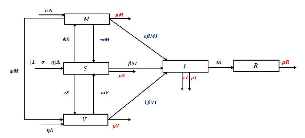
Figure 1 Flowchart of the interactions that exist among the different compartments in the model.
2.2 Mathematical Model
Here, we combine all assumptions. The proposed mathematical model with non-negative initial conditions is given by Eq. (1):
\[\begin{split} \frac{dS}{dt} &= (1 - \sigma - \eta)\Lambda + \varpi M + \omega V - (\beta I + \psi + \gamma + \mu)S, \\ \frac{dM}{dt} &= \Lambda \sigma + \psi S - (\varpi + \varepsilon \beta I + \varphi + \mu)M, \\ \frac{dV}{dt} &= \Lambda \eta + \gamma S + \varphi M - (\xi \beta I + \omega + \mu)V, \end{split}\]
\[\frac{dI}{dt} = \beta SI + \varepsilon \beta MI + \xi \beta VI - (\tau + \kappa + \mu)I,\] \[\frac{dR}{dt} = \kappa I - \mu R.\] (1)
The details of all parameters used in Eq. (1) are presented in Table 1.
Parameters Meaning Units \(\overline{(1-\sigma-\eta)}\Lambda\)People/day Inclusion rate into susceptible compartment People/day \(\Lambda \sigma\)Inclusion rate into breastfeeding compartment People/day \(\Lambda \eta\)Inclusion rate into vaccinated compartment dav-1 Breastfeeding rate of susceptible compartment dav-1 γ Vaccination rate of susceptible compartment day-1 φ Vaccination rate of breastfeeding compartment day-1 β Effective contact rate Waning rate of maternal antibodies from breast milk day-1 \(\omega\)day-1 Waning rate of vaccine \(day^{-l}\)E Reduction in the risk of infection due to maternal antibodies day 1 ξ Reduction in the risk of infection due to vaccination τ Disease mortality rate day-1 day μ Natural death rate \(\underline{d}ay^{-1}\)
Table 1 Parameters defined in the model.
Throughout this article, we assume that the initial conditions of the model in Eq. (1) are non-negative:
Rate of flow into the removed class
\[S(0) = S_0 \ge 0\]; \(M(0) = M_0 \ge 0\); \(V(0) = V_0 \ge 0\); \(I(0) = I_0 \ge 0\); \(R(0) = R_0 \ge 0\). (2)
Since the model in Eq. (1) represents the population of all the state variables and the parameters are assumed to be positive, it will be considered as being in the invariant region below:
\[\Omega_{MV} = \left\{ (S, M, V, I, R) \in \mathbb{R}^{5}_{+} : S(t) + M(t) + V(t) + I(t) + R(t) \le \frac{\Lambda}{\mu} \right\}.\] (3)
Therefore, the solutions of the model are feasible for all t > 0 if they enter and remain in the invariant region \(\Omega_{MV}\).
2.3 Positivity and Boundedness of the Solutions
The model in Eq. (1) describes a human population and so it is important to show that it is well-posed and epidemiologically meaningful. The solutions of all the state variables must remain non-negative. First, we discuss the positivity of solutions of Eq. (1) using Theorem 2.1.
Theorem 2.1. If S(0) > 0, M(0) > 0, V(0) > 0, I(0) > 0, and R(0) > 0 then the solution set \(\{S(t), M(t), V(t), I(t), R(t)\}\) of Eq. (1) is always non-negative.
Proof. Considering the first equation of the model, it can be shown that
\[\frac{dS}{dt} = (1 - \sigma - \eta)\Lambda + \varpi M + \omega V - (\beta I + \psi + \gamma + \mu)S \ge -(\beta I + \psi + \gamma + \mu)S.\]
By separating the variables, \(\frac{dS}{dt}\) reduces to
\[\frac{dS}{S} \ge -(\beta I + \psi + \gamma + \mu)dt.\]
Integrating the above equation yields the solution
\[S(t) \ge S_0 e^{-\int_0^t (\beta I + \psi + \gamma + \mu) dS} > 0.\]
Hence, it is clear from the solution above that S(t) is positive since the initial value \(S_0\) and the exponential functions are always positive. The other equations of the model in Eq. (1) can be shown to be positive using the idea above. Hence, the solutions of Eq. (1) are positive for all values t > 0. Next, we show that the solutions of all the state variables are bounded using Theorem 2.2.
Theorem 2.2 The non-negative solutions characterized by Theorem 2.1 are bounded.
Proof. From Eq. (1), the total population at changing rate is given as
\[\frac{dP}{dt} = \frac{d}{dt}(S + M + V + I + R) = \Lambda - \mu P - \tau I. \tag{4}\]
In the absence of rotavirus infection, that is I = 0, Eq. (4) becomes
\[\frac{dP}{dt} = \frac{d}{dt}(S + M + V + I + R) = \Lambda - \mu P. \tag{5}\]
The solution of Eq. (5) is found to be \(P(t) = \frac{\Lambda}{\mu} - \left[\frac{\Lambda - \mu P_0}{\mu}\right] e^{-\mu t}\), which implies that P(t) approaches \(\frac{\Lambda}{\mu}\) as \(t \to \infty\). The term \(\frac{\Lambda}{\mu}\) is defined as the threshold population level. This indicates that the total child population grows and asymptotically converges to \(\frac{\Lambda}{\mu}\). Therefore, \(\frac{\Lambda}{\mu}\) is the upper bound of the total child population P(t). If the initial child population starts below \(\frac{\Lambda}{\mu}\), then it grows over time and reaches the upper asymptotic value \(\frac{\Lambda}{\mu}\). On the other hand, if the initial population
starts higher than \(\frac{\Lambda}{\mu}\), then it decays over time and finally reaches the lower asymptotic value \(\frac{\Lambda}{\mu}\). Hence, the model in Eq. (1) is well-posed and epidemiologically meaningful.
3 Model Analysis
In model in Eq. (1) we can see that there is no term R in the first four equations. Therefore, a new model without the compartment R was considered for the model analysis in this study. This is given by Eq. (6) with non-negative initial conditions as follows:
\[\frac{dS}{dt} = (1 - \sigma - \eta)\Lambda + \varpi M + \omega V - (\beta I + \psi + \gamma + \mu)S,\] \[\frac{dM}{dt} = \Lambda \sigma + \psi S - (\varphi + \varepsilon \beta I + \varpi + \mu)M,\] \[\frac{dV}{dt} = \Lambda \eta + \gamma S + \varphi M - (\xi \beta I + \omega + \mu)V,\] \[\frac{dI}{dt} = (\beta S + \varepsilon \beta M + \xi \beta V - (\tau + \kappa + \mu))I.\] (6)
3.1 Equilibrium Points
For analysis of the model in Eq. (6), we start by computing the equilibrium points associated with Eq. (6) by setting the derivatives of each compartment to zero as follows:
\[\frac{dS}{dt} = \frac{dM}{dt} = \frac{dV}{dt} = \frac{dI}{dt} = 0. {(7)}\]
From Eq. (7), there are several equilibrium points related to Eq. (6). Here, we will consider two equilibrium points associated with epidemiology: the disease-free equilibrium point (DFE) and the endemic equilibrium point (EEP).
3.1.1 The Disease-Free Equilibrium Point (DFE)
The DFE state of the model in Eq. (6) is its steady-state solutions with the absence of rotavirus infection. In this study, the DFE state is denoted by \(E^0 = (S^0, M^0, V^0, 0)\), where
\[S^{0} = \frac{\Lambda \Big[ (\varphi + \mu + \varpi)(\mu + \omega - \mu \eta) - (\mu + \varphi + \omega)\mu \sigma \Big]}{K_{0}},\]
\[M^{0} = \frac{\Lambda \left[ (\omega + \mu + \gamma)\sigma\mu + (\mu + \omega - \mu\eta)\psi \right]}{K_{0}},\] \[V^{0} = \frac{\Lambda \left[ (\varphi + \mu + \varpi + \psi)\mu\eta + (\mu\sigma + \gamma + \psi)\varphi + (\mu - \mu\sigma + \varpi)\gamma \right]}{K_{0}},\] and \[K_{0} = \mu \left[ (\omega + \mu + \gamma)\varpi + (\varphi + \mu)(\psi + \gamma + \omega + \mu) + \psi\omega \right].\] (8)
3.1.2 The Basic Reproduction Number (BRN)
The basic reproduction number (BRN) is one of the most widely used epidemiological measurements to explore the likely spread of a virus in a given population [19]. In this study, we define the BRN of Eq. (6), denoted by \(R_{vm}\), as the number of secondary cases of rotavirus infection arising from one individual infected with the rotavirus in the presence of breastfeeding and vaccination. In the absence of vaccination and breastfeeding, BRN is denoted as \(R_0\). Using the next-generation matrix approach [20] we can create vectors \(\mathcal{F}\) and \(\mathcal{V}\), where \(\mathcal{F}\) represents the inflow and \(\mathcal{V}\) denotes the outflow of infections in the compartments of the model in Eq. (6). This is given as follows:
\[\mathcal{F} = \begin{pmatrix} 0 \\ 0 \\ \beta I(S + \varepsilon M + \xi V) \end{pmatrix} \text{ and } \mathcal{V} = \begin{pmatrix} -\Lambda \sigma - \psi S + (\varphi + \varepsilon \beta I + \varpi + \mu) M \\ -\Lambda \eta - \gamma S - \varphi M + (\xi \beta I + \omega + \mu) V \\ (\tau + \kappa + \mu) I \end{pmatrix}.\]
Next, we compute the Jacobian F from \(\mathcal{F}\) and V from \(\mathcal{V}\), respectively, to obtain
\[F = \begin{pmatrix} 0 & 0 & 0 \\ 0 & 0 & 0 \\ \varepsilon \beta I & \xi \beta I & (\beta S + \varepsilon \beta M + \xi \beta V) \end{pmatrix} \text{ and } V = \begin{pmatrix} \varphi + \varepsilon \beta I + \varpi + \mu & 0 & \varepsilon \beta M \\ -\varphi & \xi \beta I + \omega + \mu & \xi \beta V \\ 0 & 0 & \tau + \kappa + \mu \end{pmatrix}.\]
Jacobian matrices F and V evaluated at \(E^0\) yield:
\[F = \begin{pmatrix} 0 & 0 & 0 \\ 0 & 0 & 0 \\ 0 & 0 & \beta(S^0 + \varepsilon M^0 + \xi V^0) \end{pmatrix} \text{ and } V = \begin{pmatrix} \varphi + \varpi + \mu & 0 & \varepsilon \beta M^0 \\ -\varphi & \omega + \mu & \xi \beta V^0 \\ 0 & 0 & \tau + \kappa + \mu \end{pmatrix}.\]
Therefore, the BRN of the model in Eq. (6), denoted by \(R_{vm}\), is given as:
\[R_{vm} = \rho(FV^{-1}) = \frac{\Lambda\beta}{\mu(\tau + \kappa + \mu)} (S^0 + \varepsilon M^0 + \xi V^0)\] (9)
where \(S^0\), \(M^0\) and \(V^0\) are presented by Eq. (8) and \(\rho(FV^{-1})\) is the spectral radius of matrix \(FV^{-1}\). From Eq. (9) we can obtain the basic reproduction number in absence of breastfeeding and vaccination, \(R_0\), by setting the parameters related to breastfeeding and vaccination in Eq. (9) to zero. Thus, by setting \(\sigma = \psi = \varpi = \eta = \gamma = \omega = \varphi = 0\), we obtain
\[R_0 = \frac{\Lambda \beta}{\mu(\tau + \kappa + \mu)}. (10)\]
In order to explore the efficacy of controls used in this study, the relationship between \(R_{vm}\) and \(R_0\) can be derived by setting Eq. (10) into Eq. (9). Thus, we obtain
\[R_{vm} = \left[ S^0 + \varepsilon M^0 + \xi V^0 \right] R_0. \tag{11}\]
Hence, we can conclude that both breastfeeding and vaccination will be effective in preventing rotavirus infections. Hence, \(R_{vm}\) is the required BRN for our model. If \(R_{vm} < 1\), then there will be no spread of the rotavirus within the population, however, in the case where \(R_{vm} > 1\) then the disease exists within the population.
3.1.3 The Endemic Equilibrium Point (EEP)
The EEP is the point where an infection cannot be totally eliminated from a population. In our study, the EEP \(E^*\), is obtained by setting the model in Eq. (6) to zero. We denote the EEP as \(E^* = (S^*, M^*, V^*, I^*)\), where \(S^*\) represents the susceptible compartment, \(M^*\) denotes the breastfeeding compartment, \(V^*\) represents the vaccinated compartment, and \(I^*\) represents the infected compartment when \(I \neq 0\). The existence of an EEP is established in this study using Lemma 3.1.
Lemma 3.1. If \(R_{vm} > 1\), then there exists a positive endemic equilibrium point.
Proof. At endemic equilibrium point, the model in Eq. (6) becomes
\[(1 - \sigma - \eta)\Lambda + \varpi M^* + \omega V^* - (\beta I^* + \psi + \gamma + \mu)S^* = 0,\] \[\Lambda \sigma + \psi S^* - (\varpi + \varepsilon \beta I^* + \varphi + \mu)M^* = 0,\] \[\Lambda \eta + \gamma S^* + \varphi M^* - (\xi \beta I^* + \omega + \mu)V^* = 0,\] \[\beta S^* I^* + \varepsilon \beta M^* I^* + \xi \beta V^* I^* - (\tau + \kappa + \mu)I^* = 0.\] (12)
From Eq. (12), we obtain the following implicit solutions to the respective compartments,
\[S^* = \frac{(1 - \sigma - \eta)\Lambda + \omega V^* + \varpi M^*}{(\beta I^* + \psi + \gamma + \mu)}, M^* = \frac{\Lambda \sigma + \psi S^*}{(\varphi + \varepsilon \beta I^* + \varpi + \mu)} \text{ and } V^* = \frac{\Lambda \eta + \gamma S^* + \varphi M^*}{(\xi \beta I^* + \omega + \mu)}.\] where \(I^*\) is the solution of the following general cubic polynomial equation:
\[F_1 I^{*3} + F_2 I^{*2} + F_3 I^{*} + F_4 = 0, (13)\] with \(F_1\), \(F_2\), \(F_3\) and \(F_4\), given as follows:
\[F_{1} = \varepsilon \xi (\tau + \kappa + \mu),\]
\[F_{\gamma} = (\tau + \kappa + \mu)(\mu\varepsilon\xi + \varepsilon\xi\psi + \varepsilon\xi\gamma + \mu\varepsilon + \mu\xi + \varphi\xi + \varepsilon\omega + \xi\varpi) - \Lambda\beta\varepsilon\xi,\]
\[\begin{split} F_3 &= (\tau + \kappa + \mu)(\varphi\omega + \varpi\omega + \mu\varphi + \xi\gamma\varpi + \mu\xi\gamma + \varphi\xi\psi + \mu\xi\psi + \varepsilon\psi\omega \\ &+ \mu^2\xi + \mu\varepsilon\gamma + \mu\varepsilon\omega + \mu\xi\varpi + \mu\varpi + \mu\omega + \mu\varphi\xi + \mu^2 + \varphi\xi\gamma + \mu^2\varepsilon + \mu\varepsilon\psi) \\ &- \beta\Lambda \Big( \mu\sigma\varepsilon\xi + \mun\varepsilon\xi - \mu\sigma\xi - \mun\varepsilon + \varepsilon\xi\psi + \varepsilon\xi\gamma + \mu\varepsilon + \mu\xi + \varphi\xi + \varepsilon\omega + \xi\varpi \Big). \end{split}\]
\[\begin{split} F_4 &= (\tau + \kappa + \mu)(\mu \varphi \psi + \mu \varphi \omega + \mu^2 (\gamma + \varpi + \varphi + \varpi \omega + \mu + \psi + \omega) + \mu \psi \omega + \mu \gamma \varpi + \mu \varphi \gamma) \\ &- \beta \Lambda \Big( \mu^2 (1 + \sigma \varepsilon + \eta \xi - (\eta + \sigma)) + \mu \omega + \varepsilon \psi \omega + \varphi \omega + \varpi \omega + \sigma \varepsilon \omega - \mu \eta \varepsilon \psi - \mu \varphi \eta - \mu \eta \varpi \\ &+ \mu \xi \gamma + \varphi \xi \gamma + \xi \gamma \varpi + \mu \eta \xi \psi + \mu \eta \xi \varpi + \mu \varphi \eta \xi + \mu \sigma \varepsilon \gamma + \mu \varphi \sigma \xi - \mu \varphi \sigma - \mu \sigma \xi \gamma - \mu \sigma \omega \\ &+ \mu \varepsilon \psi + \mu \varphi + \mu \varpi + \varphi \xi \psi \Big). \end{split}\]
Thus, from the above expressions we can see that only \(F_1\) is positive. Due to the number of terms in \(F_2\) and \(F_3\), respectively, we cannot say with certainty that they are either positive or negative. However, for \(F_4\), its sign can be determined by comparing the terms in \(F_4\) with the condition \(R_{vm} > 1\). Recall that \(R_{vm}\) is given in Eq. (9). The terms in the inequality \(R_{vm} > 1\) are large. Thus, \(R_{vm} > 1\) can be rewritten in the following simplified form:
\[Q_5 > Q_6, \tag{14}\] where
\[Q_{\rm S} = \beta \Lambda \Big[ \mu \omega + \mu^2 + \varepsilon \psi \omega + \varphi \omega + \varpi \omega + \mu^2 \sigma \varepsilon + \sigma \xi \omega + \mu \xi \gamma + \varphi \xi \gamma + \xi \gamma \varpi + \mu^2 \eta \xi + \mu \eta \xi \psi \\ + \mu \varphi \eta \xi + \mu \eta \xi \varpi + \mu \sigma \varepsilon \gamma + \mu \varphi \sigma \xi + \mu \varepsilon \psi + \mu \varphi + \mu \varpi + \varphi \xi \psi \Big],\]
\[Q_{6} = \mu \Big[ \beta \Lambda \eta \varepsilon \psi + \beta \Lambda \varphi \eta + \beta \Lambda \varphi \sigma + \beta \Lambda \eta \varpi + \beta \Lambda \sigma \xi \gamma + \beta \Lambda \sigma \omega + \beta \Lambda \mu \eta + \beta \Lambda \mu \sigma \\ + \Big( \tau + \kappa + \mu \Big( \mu ((\omega + \mu + \gamma) \varpi + (\psi + \gamma + \omega + \mu)(\varphi + \mu) \psi \omega) \Big) \Big].\]
Hence, from the inequality in Eq. (14), if \(R_{vm} > 1\), then \(F_4 < 0\). So, \(F_4\) is negative. To find out the signs of \(F_2\) and \(F_3\), respectively, the cubic solution
given in Eq. (13) is analyzed using the Descartes rule of sign change [21]. The result of our analysis is provided in Table 2.
| Table 2 Anal | ysis of the cubi | c polynomia | l using the Descarte | s rule of sign change. |
|---|---|---|---|---|
| Cases | \(F_1\) | \(F_2\) | \(F_3\) | \(F_4\) | \(R_{vm}\) | No. of sign changes | No. of positive roots |
|---|---|---|---|---|---|---|---|
| 1 | + | + | + | - | \(R_{vm} > 1\) | 1 | 1 |
| 2 | + | + | - | - | \(R_{vm} > 1\) | 1 | 1 |
| 3 | + | - | + | - | \(R_{vm} > 1\) | 3 | 1,3 |
| 4 | + | - | - | - | \(R_{vm} > 1\) | 1 | 1 |
From the analysis carried out in Table 2, the model in Eq. (6) has a unique endemic equilibrium point if \(R_{vm} > 1\) and Cases 1, 2 and 4 in Table 2 are satisfied. Also, the model in Eq. (6) could have more than one endemic equilibrium point if \(R_{vm} > 1\) and Case 3 is satisfied. Hence, we can conclude that the model in Eq. (6) will always have an endemic equilibrium point whenever \(R_{vm} > 1\).
3.2 Stability Analysis
The global stability analysis of the model in Eq. (6) will be discussed in this section.
3.2.1 Global Stability Analysis (GSA) of DFE
Theorem 3.2. Using the standard comparison theorem, the DFE of the model in Eq. (6) is globally asymptotically stable whenever \(R_{vm} < 1\).
Proof. From section 3.1.2 we recall that the rate of variable changes in the model in Eq. (6) denoting the movement of infection occurs between compartments M, V, and I. Rewriting these variables by following the study of Huo and Feng [22], we obtain
\[\begin{bmatrix} \frac{dM}{dt} \\ \frac{dV}{dt} \\ \frac{dI}{dt} \end{bmatrix} = (F - V) \begin{vmatrix} M \\ V \\ I \end{vmatrix} - N_1 A_6 \begin{vmatrix} M \\ V \\ I \end{vmatrix} - N_2 A_7 \begin{vmatrix} M \\ V \\ I \end{vmatrix} - N_3 A_8 \begin{vmatrix} M \\ V \\ I \end{vmatrix}, \tag{15}\] where F and V are presented in section 3.1.2, respectively, \(N_1 = S^0 - S\), \(N_2 = M^0 - M\), \(N_3 = V^0 - V\),
\[A_{6} = \begin{pmatrix} 0 & 0 & 0 \\ 0 & 0 & 0 \\ 0 & 0 & \beta \end{pmatrix}, A_{7} = \begin{pmatrix} 0 & 0 & 0 \\ 0 & 0 & 0 \\ 0 & 0 & \varepsilon \beta \end{pmatrix}, \quad \text{and} \quad A_{8} = \begin{pmatrix} 0 & 0 & 0 \\ 0 & 0 & 0 \\ 0 & 0 & \xi \beta \end{pmatrix} \quad \text{are non-negative}\]
matrices.
Note that \(S^0\), \(M^0\), \(V^0\) are given in Eq. (8). The region \(\Omega_{MV}\) remains positive for all parameters in the model in Eq. (6), therefore from Eq. (15) it follows that
\[\begin{bmatrix} \frac{dM}{dt} \\ \frac{dV}{dt} \\ \frac{dI}{dt} \end{bmatrix} \le (F - V) \begin{bmatrix} M \\ V \\ I \end{bmatrix}.\] (16)
Therefore,
\[F - V = \begin{bmatrix} -(\varphi + \varpi + \mu) & 0 & -\varepsilon \beta M^{0} \\ \varphi & -(\omega + \mu) & -\xi \beta V^{0} \\ 0 & 0 & B_{11} - B_{12} \end{bmatrix}, \tag{17}\] where \(B_{11} = BS^0 + \epsilon \beta M^0 + \xi \beta V^0\) and \(B_{12} = \tau + \kappa + \mu\).
The eigenvalues associated with Eq. (17) are \(\lambda_1 = -(\omega + \mu)\), \(\lambda_2 = -(\varphi + \varpi + \mu)\), and \(\lambda_3 = -(\tau + \kappa + \mu - \beta(S^0 + \epsilon M^0 + \xi V^0))\), respectively. All eigenvalues of Eq. (17) have negative real parts, therefore (16) is stable for \(R_{vm} < 1\).
Hence, (M,V,I)=(0,0,0) as \(t\to\infty\) by the comparison theorem [23], (S,M,V,I)=(0,0,0,0) as \(t\to\infty\) and \(S\to S^0\), \(M\to M^0\), \(V\to V^0\), \(I\to 0\) as \(t\to\infty\). Hence \((S,M,V,I)\to E^0\) as \(t\to\infty\). So, \(E^0\) is globally asymptotically stable for \(R_{vm}<1\).
3.2.2 Global Stability Analysis (GSA) of DFE
In this subsection, the global asymptotic stability of \(E^*\) is discussed by using Lyapunov's direct method. From the model in Eq. (6), we constructed a common quadratic Lyapunov function using the idea of De Leon [24].
Theorem 3.3. If \(R_{vm} > 1\), then the endemic equilibrium point \(E^*\) of model (6) is globally asymptotically stable in the interior of region \(\Omega_{MV}\).
Proof. First we define \(W:\{(S,M,V,I)\in\Omega_{_{MV}}:S,M,V,I>0\}\to\mathbb{R}\).
By constructing a common quadratic function using Eq. (6), we obtain:
\[W(S, M, V, I) = \frac{1}{2} \left[ (S - S^*) + (M - M^*) + (V - V^*) + (I - I^*) \right]^2\] (18)
Then W is \(C^1\) in the interior of \(\Omega_{MV}\), where \(E^*\) denotes the global minimum of W on \(\Omega_{MV}\) hand \(W(S^*, M^*, V^*, I^*) = 0\).
Differentiating W along the solutions of the model in Eq. (6), we obtain
\[\frac{\partial W}{\partial t} = \left[ (S - S^*) + (M - M^*) + (V - V^*) + (I - I^*) \right] \frac{d}{dt} (S + M + V + I), \quad (19)\] where
\[\frac{d}{dt}(S+M+V+I) = \Lambda - \mu(S+M+V+I) - (\tau + \kappa)I.\]
Thus, Eq. (19) becomes:
\[\frac{\partial W}{\partial t} = \left[ \left( S - S^* \right) + \left( M - M^* \right) + \left( V - V^* \right) + \left( I - I^* \right) \right] \times \left( \Lambda - \mu \left( S + M + V + I \right) - \left( \tau + \kappa \right) I \right). \tag{20}\]
At the equilibrium point \(E^*\), \(\Lambda\) in Eq. (20) becomes \(\Lambda = \mu(S^* + M^* + V^* + I^*) + (\tau + \kappa)I^*\). Therefore, Eq. (20) can be rewritten as
\[\frac{\partial W}{\partial t} = \left[ \left( S - S^{\dagger} \right) + \left( M - M^{\dagger} \right) + \left( V - V^{\dagger} \right) + \left( I - I^{\dagger} \right) \right] \times \left( \mu \left( S^{\dagger} + M^{\dagger} + V^{\dagger} + I^{\dagger} \right) - \mu \left( S + M + V + I \right) + \left( \tau + \kappa \right) I^{\dagger} - \left( \tau + \kappa \right) I \right). \tag{21}\]
From Eq. (21) we have obtained
\[\frac{\partial W}{\partial t} = \left[ \left( S - S^* \right) + \left( M - M^* \right) + \left( V - V^* \right) + \left( I - I^* \right) \right] \\ \times \left( -\mu \left[ \left( S - S^* \right) + \left( M - M^* \right) + \left( V - V^* \right) + \left( I - I^* \right) \right] - (\tau + \kappa) (I - I^*) \right) \tag{22}\]
Let
\[A_{1} = S - S^{*},\]
\(A_{2} = M - M^{*},\)
\(A_{3} = V - V^{*},\)
\[A_4 = I - I^*,\] \[A_5 = A_1 + A_2 + A_3 + A_4.\]
Thus, Eq. (22) becomes
\[\frac{\partial W}{\partial t} = A_5 \left[ -\mu A_5 - (\tau + \kappa) A_4 \right]. \tag{23}\]
We can rewrite Eq. (23) to obtain
\[\frac{\partial W}{\partial t} = -\left[\mu A_5^2 + (\tau + \kappa) A_4 A_5\right]. \tag{24}\]
Hence
\[\frac{\partial W}{\partial t} = -\left[\mu A_5^2 + (\tau + \kappa) A_4 A_5\right] \le 0. \tag{25}\]
Also, \(\frac{\partial W}{\partial t} = 0\) if \(S = S^*\), \(M = M^*\), \(V = V^*\) and \(I = I^*\) in Eq. (22). Therefore, the largest compact invariant set in \((S, M, V, I) \in \Omega_{MV}\): \(\frac{\partial W}{\partial t} = 0\) is the singleton \(E^*\), where \(E^*\) is the EEP. By Lasalle's invariance principle, \(E^*\) is globally asymptotically stable in the interior of \(\Omega_{MV}\).
4 Model Analysis
A numerical analysis was performed using the model in Eq. (6) to support our model analysis. The numerical simulations were carried out using the deSolve package [26] with the fourth-order Runge-Kutta method in RStudio programming software version 1.1.442. Our simulations focused on the following three cases: Case 1 illustrates the numerical interpretation of the disease-free and endemic equilibrium points; Case 2 compares breastfeeding against both breastfeeding and vaccination to control rotavirus epidemics; and Case 3 was used to find out how well the model in Eq. (6) fits with real data. To validate our results, we consider the initial conditions as follows:
\[S(0) = 2,000, M(0) = 1,500, V(0) = 1,500, \text{ and } I(0) = 100.\]
The list of parameter values used in the simulations for Cases 1, 2, and 3 are provided in Tables 3, 4, and 5, respectively. The numerical results are discussed in the next subsections.
Table 3 Parameter values for the numerical simulations of disease-free equilibrium point and endemic equilibrium point.
| Parameters | Parameter values for DFE | Parameter values for EEP | Reference |
|---|---|---|---|
| Λ | 6.8493 | 6.8493 | [27] |
| \(\sigma\) | 0 | 0 | - |
| η | 0 | 0 | - |
| Ψ | 4.9315 x 10⁻⁴ | \(4.9315 \times 10^{-4}\) | [28] |
| γ | 1.5852 x 10⁻³ | \(1.5852 \times 10^{-3}\) | [27] |
| \(\varphi\) | 4.2616 x 10⁻⁴ | \(4.2616 \times 10^{-4}\) | [27] |
| β | Assumed | Assumed | - |
| \(\boldsymbol{\varpi}\) | 5.4945 x 10⁻³ | \(5.4945 \times 10^{-3}\) | [29] |
| \(\omega\) | 1.3699 x 10⁻³ | \(1.3699 \times 10^{-3}\) | [30] |
| \(\varepsilon\) | 0.62 | 0.62 | [31] |
| ξ | 0.71 | 0.71 | [27] |
| τ | 4.4660 x 10⁻⁴ | \(4.4660 \times 10^{-5}\) | [32] |
| \(\mu\) | 3.6529 x 10⁻⁵ | 3.6529 x 10⁻⁵ | [27] |
| \(\kappa\) | \(8.3333 \times 10^{-2}\) | \(8.3333 \times 10^{-2}\) | [33] |
| BRN | \(R_{vm} = 0.5913 < 1\) | \(R_{vm} = 1.0204 > 1\) |
Table 4 Parameter values for the numerical simulations when only breastfeeding and the combination of breastfeeding and vaccination are employed to control rotavirus epidemics.
| Parameters | Parameter values for | Parameter values for | Reference | |
|---|---|---|---|---|
| rarameters | only breastfeeding | breastfeeding and vaccination | ||
| Λ | 6.8493 | 6.8493 | [27] | |
| \(\sigma\) | 0 | 0 | - | |
| η | 0 | 0 | - | |
| \(\psi\) | \(4.9315 \times 10^{-4}\) | \(4.9315 \times 10^{-4}\) | [28] | |
| γ | 0 | \(4.9315 \times 10^{-5}\) | [27] | |
| \(\varphi\) | 0 | \(4.9315 \times 10^{-5}\) | [27] | |
| β | Assumed | Assumed | - | |
| \(\sigma\) | 5.4945 x 10⁻³ | \(5.4945 \times 10^{-3}\) | [29] | |
| ω | \(1.3699 \times 10^{-3}\) | 1.3699 x 10⁻³ | [30] | |
| \(\varepsilon\) | 0.62 | 0.62 | [31] | |
| ξ | 0.62 | 0.62 | [27] | |
| \(\tau\) | \(4.4660 \times 10^{-5}\) | \(4.4660 \times 10^{-5}\) | [32] | |
| \(\mu\) | 3.6529 x 10⁻⁵ | \(3.6529 \times 10^{-5}\) | [27] | |
| \(\kappa\) | \(8.3333 \times 10^{-2}\) | \(8.3333 \times 10^{-2}\) | [33] | |
| BRN | \(R_{vm} = 0.7482 < 1\) | \(R_{vm} = 0.7392 < 1\) | ||
| Parameters | Parameter values vaccination period | Parameter values non- vaccination period | Units | Reference |
|---|---|---|---|---|
| Λ | 13.6986 | 13.6986 | People/day | [27] |
| \(\sigma\) | 0.18 | 0.18 | People/day | [27] |
| η | 0.2669 | 0.2669 | People/day | [27] |
| Ψ | \(2.2756 \times 10^{-4}\) | \(2.2756 \times 10^{-4}\) | day-1 | [28] |
| γ | \(3.8191 \times 10^{-4}\) | 0 | day-1 | [27] |
| \(\varphi\) | 0 | 0 | day-1 | - |
| β | Assumed | Assumed | - | - |
| \(\sigma\) | \(5.4945 \times 10^{-3}\) | \(5.4945 \times 10^{-3}\) | day-1 | [29] |
| \(\omega\) | \(1.3699 \times 10^{-3}\) | \(1.3699 \times 10^{-3}\) | day-1 | [30] |
| \(\varepsilon\) | 0.62 | 0.62 | day-1 | [31] |
| ξ | 0.71 | 0.71 | day-1 | [27] |
| τ | \(4.4660 \times 10^{-5}\) | \(4.4660 \times 10^{-5}\) | day-1 | [32] |
| \(\mu\) | \(3.6529 \times 10^{-5}\) | \(3.6529 \times 10^{-5}\) | day-1 | [27] |
| κ | 8.3333x10⁻² | \(8.3333x10^{-2}\) | day-1 | [33] |
Table 5 Parameter values to fit the model with real data.
4.1 Numerical Interpretation of the DFE
The numerical result obtained from the numerical simulation of the disease-free equilibrium when \(R_{vm} = 0.5913 < 1\) is given in Figure 2.
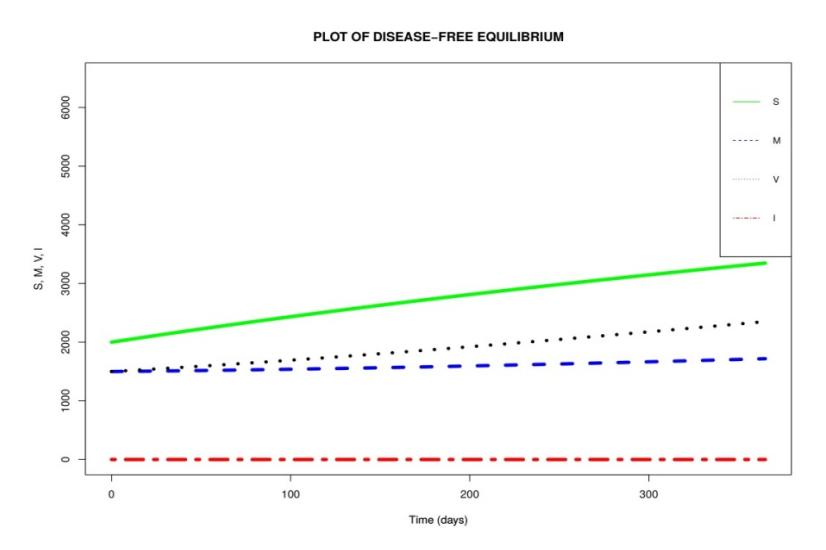
Figure 2 Simulation results of the disease-free equilibrium for the model in Eq. (6) at different initial conditions and parameter values in Table 3 when \(R_{vm} = 0.5913 < 1\).
In Figure 2, we notice a rise in the number of susceptible children in the absence of infection. We also note that when the number of susceptible children increases, the number of vaccinated and breastfeeding children increases as well. This could be due to the fact that in the absence of infection (i.e. I = 0)
there will be no children to spread the disease. This leads to a rise in the number of children in other compartments.
4.2 Numerical Interpretation of the EEP
The numerical result obtained from the numerical simulation of the endemic equilibrium when ௩ ൌ 1.0204 1 is given in Figure 3.
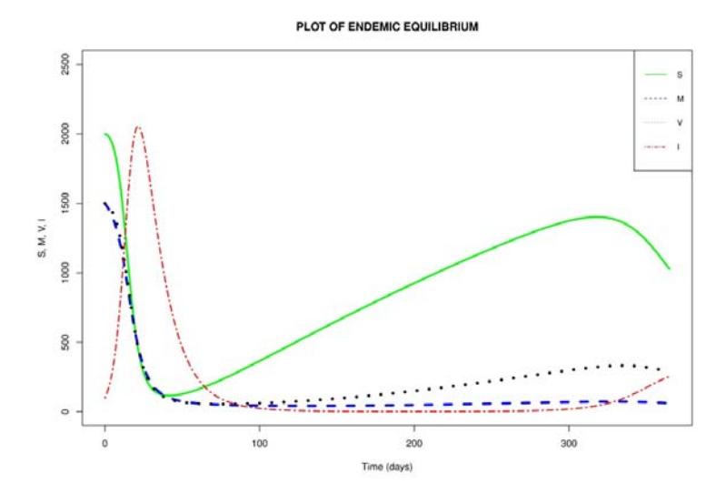
Figure 3 Simulation results of the endemic equilibrium for the model in Eq. (6) at different initial conditions and parameter values in Table 3, when ௩ ൌ 1.0204 1.
Figure 3 shows an initial rise in the number of children infected with the rotavirus. The infection peaks at 40 days. After the peak of infection, fewer children were infected, leading to a rise in the number of children in the susceptible, vaccinated, and breastfeeding compartments, respectively. A small rise in infection is noticed from about 300 days upwards. However, the number of infected children was not high when compared with the number of infections recorded in the early infection phase. Furthermore, we also notice that whenever there was a dip in infection there was a rise in the number of children in the susceptible compartment. Thus, an outbreak of rotavirus infection can spread quickly if it is not properly monitored or controlled.
4.3 Effects of Breastfeeding and Vaccination on Rotavirus Infection
In order to understand the effects of breastfeeding and vaccination on rotavirus epidemics, two scenarios were considered. The first scenario is when only breastfeeding is used as control for a rotavirus epidemic in a community. The second scenario is the introduction of vaccination in a community that already employs breastfeeding to control the rotavirus. The parameter values in Table 4 were used for the simulation. From Table 4, three parameters, namely ψ, φ and γ, are of particular interest. As earlier defined in Section 2.1, ψ represents the breastfeeding rate of the susceptible population, φ denotes the vaccination rate of the breastfeeding population, and γ stands for the vaccination rate of the susceptible population. To examine both scenarios differently, the parameter values ൌ 4.9315 ൈ 10ିସ, ൌ0 and ൌ0 were used for the first scenario. For the second scenario, one-tenth of ψ was the value used for ൌ 4.9315 ൈ 10ିହand ൌ 4.9315 ൈ 10ିହ respectively.
The one-tenth used to obtain the value of φ and γ was based on the assumption that the vaccination rate is only one-tenth of the breastfeeding rate. By computing the basic reproduction numbers using the parameter values in Table 4, we found that the combination of breastfeeding and vaccination (Scenario 2) with ௩ ൌ 0.7392 is more effective to control rotavirus epidemics than only breastfeeding (scenario 1) with ௩ ൌ 0.7482. This is an indication that the introduction of vaccination in a community that employs breastfeeding to control the rotavirus yields a more positive result than by only breastfeeding.
4.4 Comparison of Real Data and Simulated Data
In this section, we fit the real data given in Table 6 with the model in Eq. (6). The data were recorded monthly and obtained from the study of Tharmaphornpilas, et al. [27]. The data span September 2012 to October 2014. In the data, the children were only vaccinated from September 2012 to June 2013 (303 days). However, no vaccination occurred from July 2013 to October 2014 (488 days).
| Table 6 | Number of children who tested positive for rotavirus between | |||||
|---|---|---|---|---|---|---|
| September 2012 and October 2014. |
| Month | Number of infected children in 2012 | Number of infected children in 2013 | Number of infected children in 2014 |
|---|---|---|---|
| January | - | 13 | 24 |
| February | - | 16 | 20 |
| March | - | 31 | 5 |
| April | - | 14 | 4 |
| May | - | 9 | 2 |
| June | - | 11 | 0 |
| July | - | 9 | 0 |
| August | - | 15 | 0 |
| September | 1 | 17 | 0 |
| October | 1 | 15 | 1 |
| November | 1 | 12 | - |
| December | 3 | 2 | - |
To easily compare the real data with the simulated data, the monthly data in Table 6 were first interpolated into daily data. After the interpolation, we constructed two models from the model in Eq. (6) to accommodate both the aforementioned cases of vaccination and non-vaccination periods in the data. By using the parameter values given in Table 5 for a simulation, the result obtained from the model fit is given in Figure 4.
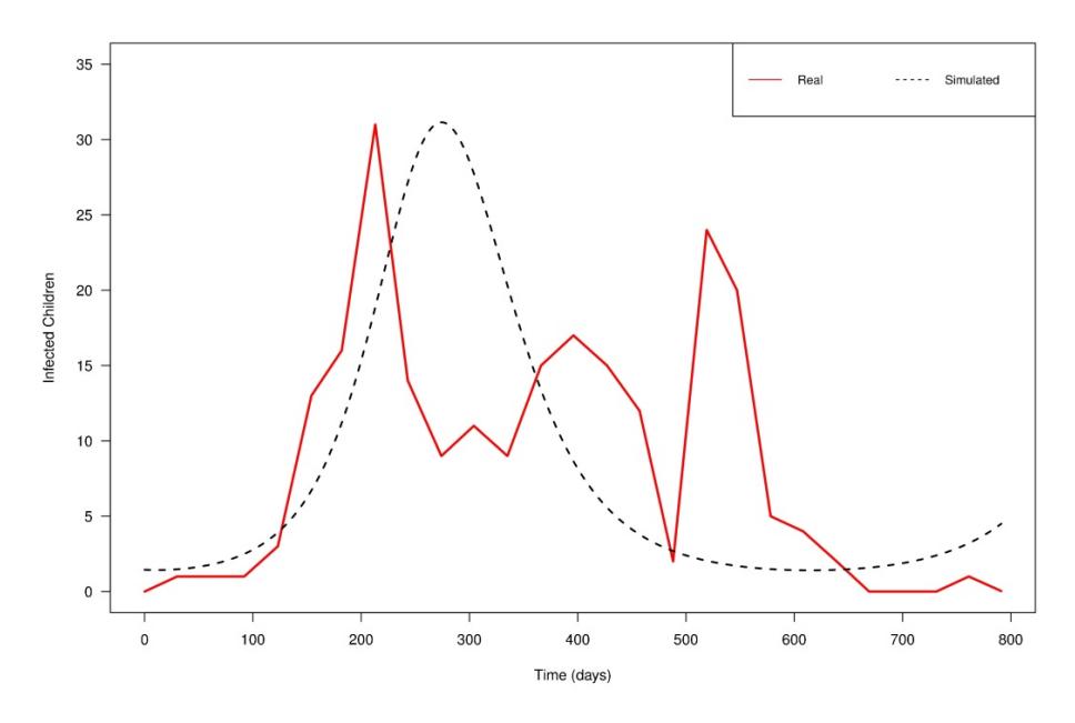
Figure 4 Comparison between real and simulated data.
From Figure 4, it can be seen that the real data have three peaks on days 213, 396, and 521, respectively. However, for the simulated data, we were only able to generate one peak, on day 275, which appears to fit well with the highest (first) peak obtained in the real data. The reasons why we were unable to generate the other two peaks in the real data using the simulated data may be the following. Firstly, our model considered a constant vaccination rate for children during the vaccination period between September 2012 and June 2013. However, in real life this may not have been the case since the number of children who go for vaccination on one day is often not the same. Next, the children tested positive in the data were children who visited the hospital. There may have been a situation whereby some other children were infected but they did not report to the hospital. Hence, the data used in this study may have been under-reported. Finally, the model proposed in this study assumes that breastfeeding and vaccination can control rotavirus infection. However, in reality, the evidence for the protective ability offered by breastfeeding against rotavirus infection remains inconclusive.
5 Conclusion
In this study, a nonlinear mathematical model was formulated and analyzed to examine the effects of breastfeeding and vaccination on the transmission dynamics of rotavirus epidemics. We have shown that the model has two possible equilibrium points, namely the disease-free equilibrium point and the endemic equilibrium point. We have computed the basic reproduction number denoted as ௩ and have further shown that if ௩ ൏ 1, then the infection will die out. However, if ௩ 1, then the infection will remain in the population. Additionally, we have shown that both the disease-free equilibrium and the endemic equilibrium are globally asymptotically stable under some specific conditions. Numerical simulations have been performed to support the analytic results. Also, real data were fitted to the model for predicting the infected population in real life. Our model showed that the combination of both breastfeeding and vaccination is more effective in reducing the spread of the rotavirus.
Although at present lower vaccine efficacy is experienced in high-mortality nations, there are approaches in various rotavirus vaccine research centers to improve the current vaccines. Some of these approaches include modifying or developing new vaccine formulations, altering the schedules of existing rotavirus immunizations, and increasing the number of vaccine doses given to children [11]. Thus, we hope that when the current vaccines are improved in the future, developing countries will experience a higher rotavirus vaccine efficacy to help control rotavirus epidemics.
Acknowledgements
This work was supported by the Higher Education Research Promotion and the Thailand's Education Hub for Southern Region of ASEAN Countries Project Office of the Higher Education Commission. We would also like to thank the editor and anonymous reviewers for their thoughtful comments. In addition, we are grateful to Dr. Tatdow Pansombut and Assoc. Prof. Dr. Aniruth Phon-on of the Department of Mathematics and Computer Science, Prince of Songkla University, Pattani Campus, Pattani, for their valuable suggestions and inputs in this article.