1 Introduction

Nonlinear problems are of great interest to engineers, physicists, mathematicians and many other scientists. The natural behavior of nonlinear systems is described in mathematics by a system nonlinear of equations. Consider the nonlinear system

\[g(x) = 0, (1)\] where the function \(g:R^r\to R^n\) is a continuously differentiable. The system is described as an overdetermined system when \(n\geq r\), and classified as underdetermined when \(r\geq n\). Moreover, when n=r, then the system is referred to as a square nonlinear system. Specifically, the system is considered to be monotone whenever

\[(g(x) - g(s))^{T}(x - s) \ge 0, \quad \forall x, s \in \mathbb{R}^{r}.\]

The purpose of this hybrid method is to provide an alternative approach for globally converging large-scale monotone equations with a smaller computational burden and less CPU time consumption without computing the

Jacobian matrix. Popular schemes for solving Eq. (1) are the Newton and quasi-Newton methods [2,4,13,14]. They use the iterate

\[x_{k+1} = x_k - (g'(x_k))^{-1} g(x_k), \quad k = 0, 1, 2, ....\] (3)

Interesting qualities of these schemes include rapid convergence and easy implementation. However, they are generally not much used for solving largescale monotone equations because they have to compute and store the Jacobian matrix or its approximation at every iteration. Conjugate gradient (CG) methods are specifically attractive due to their smaller memory requirement for largescale problems. Waziri and Sabi'u [9] developed a CG method for solving symmetric nonlinear equations. They demonstrated the global convergence for their method with the aid of a non-monotone line search. The numerical comparison indicated that their scheme is reliable and competent. In line with the literature, Cheng and Li [5] extended the prominent Hager and Zhang nonmonotone line search method [10] to solve large-scale nonlinear systems. Furthermore, a significant number of conjugate gradient methods have been proposed in the literature, among others [1-3,6,8,16-19]. Comprehensive numerical results evidenced that each method is appropriate for large-scale problems. This paper presents three-term hybrid Polak-Ribiére-Polyak (PRP) and Fletcher-Reeves (FR) CG methods for large-scale monotone equations. It is organized as follows: in Section 2 we give the details of our approach followed by the convergence result in Section 3. Numerical comparisons can be found in Section 4 and the conclusion is given in Section 5.

2 Details of the Proposed Scheme

Given a point \(x_0\), the CG method generates the following iterates:

\[x_k = x_{k-1} + \alpha_k d_{k-1}, \quad k = 1, 2...\] (4)

where the term \(d_k\) is the conjugate gradient direction and \(\alpha_k\) is the step size to be computed using typical line search (Backtracking, Armijo or Wolfe line search, and others). Let \(v_k = x_{k-1} + \alpha_k d_{k-1}\). The hyperplane

\[H_{k} = \left\{ x \in R^{r} \mid (x - v_{k})^{T} g(v_{k}) = 0 \right\}\] (5)

strictly separates \(x_k\) from the solution set of Eq. (1). From this fact Solodov and Svaiter in [7] denoted the next iterate \(x_k\) to be

\[x_{k} = x_{k-1} - \frac{g(v_{k})^{T} (x_{k-1} - v_{k})}{\|g(v_{k})\|^{2}} g(z_{k}).\] (6)

In the work of Zhang, et al. [14] the CG direction is given as

\[d_{k} = \begin{cases} -g_{k}, & \text{for } k = 0, \\ -g_{k} + \beta_{k}^{PRP} d_{k-1} - \theta_{k}^{PRP} y_{k-1}, & \text{for } k \ge 1, \end{cases}\] (7)

where \(\beta_k^{PRP} = \frac{g_k^T y_{k-1}}{\|g_{k-1}\|^2}\) and \(\theta_k^{PRP} = \frac{g_k^T d_{k-1}}{\|g_{k-1}\|^2}\). Motivated by the above ideas of

Zhang et al. [14], we present a hybrid three-term CG direction as:

Recall that from [1], \(\beta_k^{FR} = \frac{\parallel g_k \parallel^2}{\parallel g_{k-1} \parallel^2}\) and \(\theta_k^{FR} = \frac{d_{k-1}^T y_{k-1}}{\parallel g_{k-1} \parallel^2}\). Now we define our rigorous direction to be

\[d_{k} = \begin{cases} -g_{k}, & \text{if } k = 0, \\ -g_{k} + \beta_{k}^{H^{*}} d_{k-1} - \theta_{k}^{H^{*}} y_{k-1}, & \text{if } k \ge 1, \end{cases}\](8)

where

\[\beta_{k}^{H^{*}} = \frac{\min\left\{g_{k}^{T} y_{k-1}, \|g_{k}\|^{2}\right\}}{\|g_{k-1}\|^{2}}, \text{ and } \theta_{k}^{H^{*}} = \frac{\min\left\{d_{k-1}^{T} y_{k-1}, g_{k}^{T} d_{k-1}\right\}}{\|g_{k-1}\|^{2}}.\] (9)

For the computation of stepsize \(\alpha_k\), the derivative free line search used in [11] is an interesting idea. Let, \(\alpha_k = \max\{s, rs, r^2s, ...\}\), satisfying

\[-g(x_k + \alpha_k d_k)^T d_k \ge \omega \alpha_k \parallel g(x_k + \alpha_k d_k) \parallel \parallel d_k \parallel^2.\] (9)

Algorithm

Step 1: Given \(x_0, r, r\omega \in (0,1)\), set k=0 and \(d_0=-g_0\).

Step 2 : Verify the stopping conditions. If yes, then stop; else go to Step 3.

Step 3 : Use Eq. (8) to compute \(d_k\).

Step 4: Determine \(\alpha_k\) by Eq. (10).

Step 5: Compute \(x_k = x_{k-1} - \frac{g(z_k)^T (x_{k-1} - z_k)}{\|g(z_k)\|^2} g(z_k)\).

Step 6 : Allow k = k + 1 and repeat step 2.

3 Convergence Result

For our algorithm to converge globally, we assume that g is Lipschitz continous and for \(L_1, L_2 > 0\) we have

\[||g(x)|| \le L_1 \text{ and } ||g(v)|| \le L_2.\] (11)

Lemma 3.1 Assume \(g(x^*) = 0\) and \(\{x_k\}\) as obtained by our algorithm. We obtain \(\|x_{k+1} - x^*\|^2 \le \|x_k - x^*\|^2 - \|x_{k+1} - x_k\|^2\). Hence, \(\{x_k\}\) is bounded and \(\sum_{k=0}^{k=\infty} \|x_{k+1} - x_k\|^2 < \infty\).

Lemma 3.2 [8] Let \(\{x_k\}\) and \(\{v_k\}\) be computed by the proposed algorithm. We obtain

\[\alpha_{k} \geq \min \left\{ \beta_{k}^{H*}, \frac{\delta \theta}{L+, \omega \parallel g(v_{k}') \parallel} \frac{\parallel g_{k} \parallel^{2}}{\parallel d_{k} \parallel^{2}} \right\}\] \[(12)\]

Where \(z' = x_k + \alpha_k d_{k-1}\).

Theorem 3.3 Suppose \(\{x_k\}\) is obtained by our algorithm. Let \(s_k = x_k - x_{k-1}\). Then

\[\lim_{k \to \infty} \|\alpha_k d_k\| = \lim_{k \to \infty} \|s_k\| = 0, \tag{13}\]

Proof.

\[||x_{k} - x_{k-1}|| = \frac{|g(v_{k})^{T}(x_{k-1} - v_{k})|}{||g(v_{k})||} \le \frac{||g(v_{k})|| ||x_{k-1} - v_{k}||}{||g(v_{k})||}\](14)

\[= \parallel x_{\iota} - v_{\iota} \parallel = \alpha_{\iota} \parallel d_{\iota} \parallel. \tag{15}\]

Theorem 3.4 Let \(\{x_k\}\) be generated by our algorithm. Then

\[\liminf_{k \to \infty} \|g(x_k)\| = 0.\] (16)

Proof. Assume Eq. (16) does not hold, i.e.

\[||g(x_k)|| \ge \tau, \quad \forall k \ge 0.\] (17)

Clearly, \(||g_k|| \le ||d_k||\), which implies

\[\parallel d_k \parallel \geq \tau, \quad \forall k \geq 0.\] (18)

Observe that,

\[||y_k|| = ||g(x_k) - g(x_{k-1})|| \le L ||s_k||,\] (19)

from the defintion of \(\beta_k^{H*}\) we have

\[|\beta_{k}^{H^{*}}| \leq \frac{\min\{L ||s_{k}||, L_{1}\}}{L_{1}},\] (20)

Also, for \(\theta_k^{H*}\) we get

\[\mid \theta_{k}^{H^{*}} \mid \leq \frac{\min\left\{\tau L \parallel s_{k} \parallel, \tau L_{1}\right\}}{L_{1}}.\] (21)

Therefore, we let the following inequalities be true for all \(k \ge 0\). We obtain

\[\parallel d_{k} \parallel \leq \parallel g_{k} \parallel + \mid \beta_{k}^{H^{*}} \parallel \mid d_{k-1} \parallel - \mid \theta_{k}^{H^{*}} y_{k}\]

\[\leq L_{1} + \tau \frac{\min\{L \parallel s_{k} \parallel, L_{1}\}}{L_{1}} - \frac{\min\{\tau L \parallel s_{k} \parallel, \tau L_{1}\}}{L_{1}} \\ \leq L_{1} + \tau \frac{\min\{L \parallel s_{k} \parallel, L_{1}\}}{L_{1}}.\] (22)

Let \[M^* = L_1 + \tau \frac{\min\{L \parallel s_k \parallel, L_1\}}{L_1}\]. We get \(\parallel d_k \parallel \leq M^*\). (23)

This combined with Lemma 3.2 and Eq. (11) and inequalities \(||d_k|| \ge \tau\), \(||g_k|| \ge \tau\) implies for all k sufficiently large,

\[\|d_{k}\|\alpha_{k} \geq \min\left\{\beta_{k}^{H^{*}}, \frac{\delta\theta}{L+,\omega\|g(v_{k}')\|} \frac{\|g_{k}\|^{2}}{\|d_{k}\|^{2}}\right\} \|d_{k}\| > 0.\] (24)

The last inequality gives a contradiction with Eq. (17). Therefore, Eq. (16) is true and hence the proof.

4 Numerical Experiment

In this section, our algorithm is compared with the three-term Polak-Ribiére-Polyak (TPRP) CG method [6]. For both algorithms we set \(\omega = 10^{-4}\), r = 0.2 and s = 1. The code was implemented in Matlab 7.4 R2010a and run on a computer with 4 GB RAM memory capacity and a 1.8 GHz CPU processor. Iterations were stopped when the number of iterations was greater than 2000 or \(||g_k|| \le 10^{-4}\). Eleven problems were tested to demonstrate the robustness of our algorithm compared to the TPRP method.

Problem 1

\[g_{i}(x) = e^{x_{j}} - 1, \quad j = 1, 2, \dots, n\]

Problem 2

\[g_1(x) = x_1(x_1^2 + x_2^2) - 1\] \[g_j(x) = x_j(x_{j-1}^2 + 2x_j^2 + x_{j+1}^2) - 1, \quad j = 1, 2, \dots, n-1\] \[g_n(x) = x_n(x_{n-1} + x_n^2).\]

Problem 3 For \(j = 1, 2, \dots, n/3\),

\[g_{3j-2}(x) = x_{3j-2}x_{3j-1} - x_{3j}^{2} - 1,\] \[g_{3j-1}(x) = x_{3j-2}x_{3j-1}x_{3j} - x_{3j-2}^{2} + x_{3j-1}^{2} - 2,\] \[g_{3j}(x) = e^{-x_{3j-2}} - e^{-x_{3j-1}}.\]

Problem 4 For \(j = 2, 3, \dots, n-1\)

\[g_1(x) = 3x_1^3 + 2x_2 - 5 + \sin(x_1 - x_2)\sin(x_1 + x_2)\] \[g_j(x) = -x_{j-1}e^{x_{j-1}-x_j} + x_j(4 + 3x_j^2) + 2x_{j+1} + \sin(x_j - x_{j+1})\sin(x_j + x_{j+1}) - 8,\] \[g_n(x) = -x_{n-1}e^{x_{n-1}-x_n} + 4x_n - 3.\]

Problem 5

\[g_{1}(x) = x_{1} - e^{\frac{\cos(x_{1} + x_{2})}{n+1}}\] \[g_{j}(x) = x_{j} - e^{\frac{x_{j-1} + x_{j} + x_{j+1}}{n+1}}, \quad j = 2, 3, \dots, n-1\] \[g_{n}(x) = x_{n} - e^{\frac{\cos(x_{n-1} + x_{n})}{n+1}}.\]

Problem 6

\[g_1(x) = \cos(x_1) - 9 + 3x_1 + 8e^{x_2}\]
\[g_i(x) = \cos(x_i) - 9 + 3x_i + 8e^{x_{j-1}}, \quad j = 2, 3, \dots, n\]

Problem 7

\[g_j(x) = x_j^2 + (x_j - 3)\log(x_j + 3) - 9, \quad j = 1, 2, 3, \dots, n\]

Problem 8

\[g_{j}(x) = (x_{j}^{2} - 1)^{2} - 2, \quad j = 1, 2, 3, ..., n\]

Problem 9

\[g_{j}(x) = 4x_{j} + (x_{j+1} - 2x_{j}) - \frac{x_{j+1}^{2}}{3}, \quad j = 1, 2, \dots, n-1\]
\(g_{n}(x) = 4x_{n} + (x_{n-1} - 2x_{n}) - \frac{x_{n-1}^{2}}{3}.\)

Problem 10

\[g_1(x) = \sin(x_1 - x_2) - 4e^{2-x_2 + 2x_1}\] \[g_1(x) = \sin(2 - x_1) - 4ex_1 - 2 + 2x_1 + \cos(2 - x_1) - e^{(2-x_1)}, \quad j = 2, 3, \dots, n\]

Problem 11

\[g_j(x) = \sum_{j=1}^n (x_j - 2) + \cos(x_j - 2) - 1, \quad j = 1, 2, 3, \dots, n\]

From Figures 1 and 2 it can be observe that our proposed algorithm has the advantages of using less CPU time and less iterations over TPRP in almost all the eleven problems tested in our experiment using Dolan and Moré's performance profile [20].

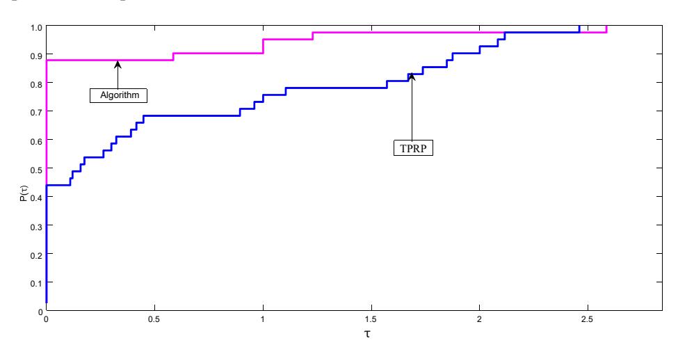
Figure 1 Performance profile of our algorithm versus the TPRP method [6] for number of iterations.

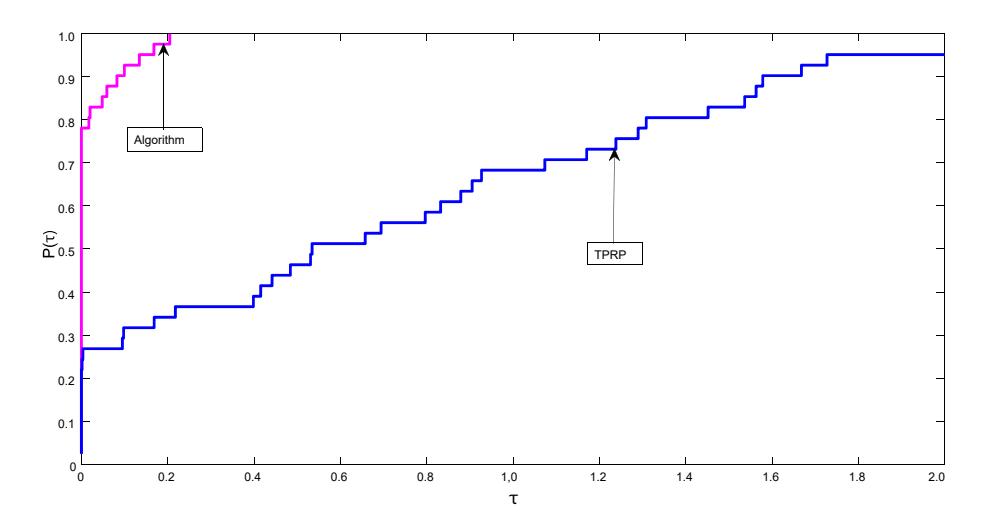
Figure 2 Performance profile of our algorithm versus the TPRP method [6] for CPU time in seconds.

5 Conclusion

This article proposes an effective new hybrid approach for solving monotone nonlinear equations with less iterations as well as less CPU time consumption without computing the Jacobian matrix. The numerical results show that this method is more efficient compared to TPRP [6]. The extension of this method to a more general system of smooth and nonsmooth equations will be investigated in a future research.

Acknowledgement

The first author is grateful to TWAS/CUI for the 2017 CUI-TWAS Full-time Postgraduate Fellowship with FR number 3240299486.