
1 Introduction
Carbon steel is a material that is used widely for oil and gas pipelines in the petroleum industry. It is easily formed and inexpensive. However, carbon steel has the shortcoming of being very susceptible to corrosion due to contact with its environment [1]. Corrosion is a serious problem in the inner surface of pipelines as media of crude oil and natural gas transportation. The mixture of crude oil and natural gas also contains dissolved salts and CO2, which are corrosive substances [2,3]. These compounds simultaneously flow from the well to the refining and storage facilities. During this transportation process, dissolved salts and CO2form chloride ions and carbonic acid, increasing the corrosion rate because they can interact with the iron as the principal material of the pipeline. This is the main cause of pipeline leakage and oil spills, which conduce serious economic losses in the petroleum industry [4]. In addition, environmental pollution also threatens to harm the ecosystem around oil spills.
Several methods are used to control the corrosion rate of pipeline materials, such as coatings, using corrosion inhibitors and corrosion-resistant materials. Corrosion inhibitors are often used to protect the inner surface of pipelines for effective and economic reasons. The use of these materials can increase the lifetime of pipelines [4,6]. On the other hand, using a corrosion-resistant material entails an unreasonable cost, for example, stainless steel [5-7].
Previous studies have explained that organic compounds containing donor atoms (N, O, S) and N-heterocyclic structures have good activity as corrosion inhibitor on carbon steel [8-10]. This is related to their ability to be adsorbed on metal surfaces. Meanwhile, the adsorption activity of organic molecules on a metal surface mainly depends on the surface charge of the metal, the chemical structure of the molecules and the aggressiveness of the solution [11]. Polysuccinimide (PSI) is a N-heterocyclic biopolymer and is known as an intermediate compound of polyaspartic acid (PASP). Both of them are nontoxic and biodegradable polymers [12,13], however, only PASP is used widely as a non-phosphorous, antiscalant and a corrosion inhibitor due to its watersoluble property, good dispersion capacity and its ability as a chelating agent that can reduce the corrosion rate and prevent the deposition of calcium carbonate, calcium phosphate and calcium sulfate on the pipeline [12-15]. The structure of PSI and PASP are displayed in Figure 1. The presence of carboxylic and amide groups in PASP's molecular structure can protect carbon steel from corrosion attacks. Meanwhile, PSI is soluble only in organic solvents such as dimethylformamide (DMF), which cause a risk of environmental damage [15]. The water insolubility is a crucial limitation of PSI for some applications, in particular as a corrosion inhibitor. Additional treatments are required to convert PSI into PASP, but these need extra chemical substances, energy, and exhaustive time.
Significant reduction in the chain length of PSI to its oligomeric form or oligosuccinimide (OSI) is expected to increase its polarity as well as its solubility in water, so it can be applied as corrosion inhibitor without converting to PASP first. Using an appropriate method is important to obtain hygroscopic OSI. Therefore, this work aimed to synthesize the OSI compound and to evaluate its performance as corrosion inhibitor in 1% NaCl solution saturated by CO2 as well as to study the adsorption isotherm and adsorption energy.
\[\text{[rumus tidak dapat ditampilkan dengan baik — lihat PDF asli]}\]
Figure 1 The structure of (a) PSI and (b) PASP [13,14].
2 Experimental
2.1 General Procedure
All reagents used in this research were analytical grade. The infrared spectra of the synthesized products were analyzed using a Fourier Transform Infrared ALPHA Bruker device. The structures of the products were elucidated based on NMR spectra obtained using a Bruker Avance 500 MHz (1H NMR) and a 125 MHz (13C NMR) spectroscope with D2O as solvent due to the hygroscopic nature of the synthesized compound. The fractions and molecular weights of all products were measured using an Acquity UPLC BEH device (C18, 1,7 µm, 2,1 x 100 mm column) aligned with an XEVO Quadrupole Time-of-Flight (QToF) mass spectrometer and eluted with gradient mobile phase of water containing 0.01% formic acid and acetonitrile at a flow rate 0.2 mL.min-1 . Electrochemical measurements of the corrosion inhibition were carried out using a Voltalab PGZ 301 device assisted by the Voltamaster 4 software. For the analysis, a threeelectrode configuration was applied that used carbon steel as working electrode, saturated calomel electrode (SCE) as reference electrode, and platinum as auxiliary electrode. The weight loss measurement was performed using a wheel test corrosion oven. The components of the carbon steel (%) were C (0.1), P (0.025), Mn (0.45), S (0.03), and balanced Fe [16].
2.2 Synthesis of Oligosuccinimide
The synthesis of oligosuccinimide was carried out according to the method proposed by Liu, et al. [12] with some modifications, by mixing 19.6 g of maleic anhydride in demineralized water and 23.06 g of ammonium carbonate, which was also dissolved in demineralized water. The mixture was refluxed for 1 hour at 180 °C. After completion of the reaction, the solvent was evaporated until an orange solid was formed. The resulting solid was washed with absolute
ethanol and dried in vacuum oven at 65 °C for 24 hours. Furthermore, the obtained oligosuccinimide was placed in a desiccator until further use.
2.3 Corrosion Test by Electrochemical Measurements
Electrochemical measurements were carried out using the electrochemical impedance spectroscopy (EIS) and potentiodynamic polarization (Tafel) techniques. The vessel was filled with 100 mL 1% (w/v) NaCl solution as blank solution for each measurement, followed by continuous sparging of CO<sub>2</sub> gasses into the vessel, and applying a magnetic stirrer throughout the experiment. The flow rate of CO<sub>2</sub> fulfillment was 150 mL.min<sup>-1</sup> and the stirring speed was 250 rpm. Measurements of each sample solution for the various temperatures were initiated by the measurement of blank solution. EIS was run at a frequency of 10 kHz to 100 mHz, with variations of system temperature at 25, 35, and 45 °C, respectively, and the variations of inhibitor concentration were 18.5, 37.0, 55.5, 74.0, and 92.5 ppm, respectively. The Tafel technique was carried out at the temperature that generated the highest efficiency from EIS within a concentration range of 55.5 to 111 ppm. The scan rate of this technique was 0.2 mV.s<sup>-1</sup> with a potential range of \(E_{corr}\) -50 mV to \(E_{corr}\) +50 mV. The efficiency of corrosion inhibition, commonly referred to as the inhibition efficiency (IE), by the EIS and Tafel techniques was calculated according to the following equations [9]:
\[IE = \frac{Rct_{inh} - Rct}{Rct_{inh}} \times 100\% \tag{1}\]
\[IE = \frac{I_{corr\,o} - I_{corr\,inh}}{I_{corr\,o}} \times 100\%\] (2)
where \(R_{ct}\) and \(R_{ct}_{inh}\) are the charge transfer resistance (\(\Omega\).cm<sup>2</sup>) without and with inhibitor, respectively, \(I_{corr\,o}\) and \(I_{corr\,inh}\) are the unprotected and protected corrosion current density (mA.cm<sup>-2</sup>) of the carbon steel electrode.
2.4 Corrosion Test by Weight Loss Measurements
In this method, the initial weight of the carbon steel sheets was measured using a digital analytical balance with a precision of \(\pm\) 0.1 mg. The contact surface area of the sheets was 5.1634 cm<sup>2</sup>. Each of them was placed into different bottles filled with 200 mL NaCl solution (1% w/v), with inhibitor (18.5, 37.0, 55.5, 74.0, and 92.5 ppm) and without inhibitor. Then, they were saturated with CO<sub>2</sub> gas before being transferred into a wheel test corrosion oven. The corrosion processes took place for 48 hours at 35 °C as the minimum temperature inside the oven, accompanied by mechanical wheel agitation. After that, each bottle was taken out of the oven and the carbon steel sheets were taken out, soaked with Clarke solution, rinsed with absolute ethanol, atmosphere dried, and their
final weights were measured. The corrosion rate and efficiency of corrosion inhibition were determined by Eq. (3) and Eq. (4) respectively.
\[C_R = \frac{24}{t} \left( \frac{365 \cdot \Delta W}{A \cdot d} \right) \cdot 10 \tag{3}\]
\[IE = \frac{c_{Ro} - c_{Ri}}{c_{Ro}} \times 100 \tag{4}\] where CR is the corrosion rate (mmPY), ∆W is the weight loss (g), A is the surface area of the carbon steel sheet (cm2 ), d is the density of carbon steel (7.86 g.cm-3 ), and t is the duration of the wheel test (hours), CRo and CRi are the corrosion rates of the system without and with inhibitors, respectively [17].
3 Results and Discussion
The synthesis of oligosuccinimide was carried out by thermal condensation with maleic anhydride and ammonium carbonate as precursors. The molar ratio used in this reaction was 1:1.2, according to the previous study performed by Liu, et al. [12], due to the highest scale inhibition of the synthesized product. This method is quite simple, inexpensive and does not require an initiator because the oligomerization reactions occur on the functional groups of each precursor to produce 32.17 g hygroscopic oligosuccinimide. Its functional groups and chemical shifts of protons and carbons were confirmed by FTIR and NMR spectroscopy, respectively. The relevant synthetic reaction is shown in Figure 2.
Figure 2 The synthesis scheme of oligosuccinimide.
3.1 Analysis of Functional Groups by FTIR Spectrophotometry
The IR spectra of the oligosuccinimide molecular structure (Figure 3) showed vibrational peaks of bonds between atoms in the functional groups of OSI molecules. There was a widening peak in the wavenumber range from 3174 to 3425 cm-1 due to stretching vibrations of -NH groups that formed hydrogen bonds [18]. Two peaks at 2957 and 3005 cm-1 showed stretching vibration of C-H from alkanes and alkenes. There was a peak at wavenumber 1717 cm-1 related to vibration of C=O imide from five-ring bonds [12]. Furthermore, the peak at wavenumber 1622 cm-1 corresponds to the vibrational bonds of carbon alkenes (C=C). The high intensity peak at wavenumber 1400 cm-1 represents bending
vibrations of C-H bond from O=C-CH2- [18] and C-N bonding vibrations [12,19,20].
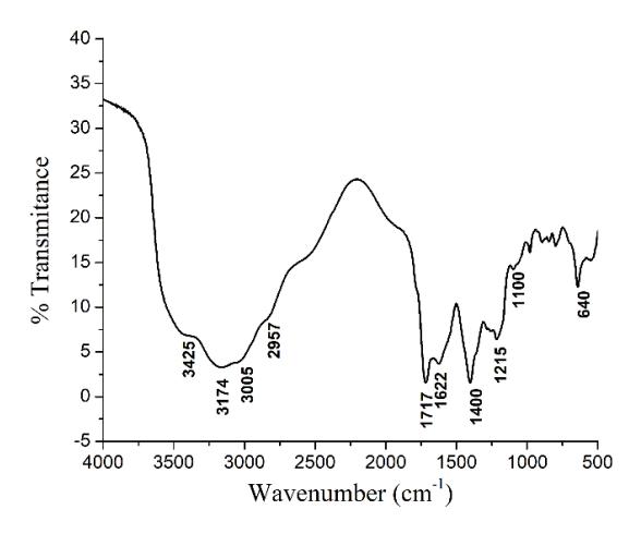
Figure 3 FTIR spectra of oligosuccinimide.
3.2 The Structure Characterization Using NMR Spectroscopy
The 1H NMR spectra of oligosuccinimide in D2O solvent is displayed in Figure 4. Some proton signals and their chemical shifts showed the presence of proton types in the synthesized OSI compound.
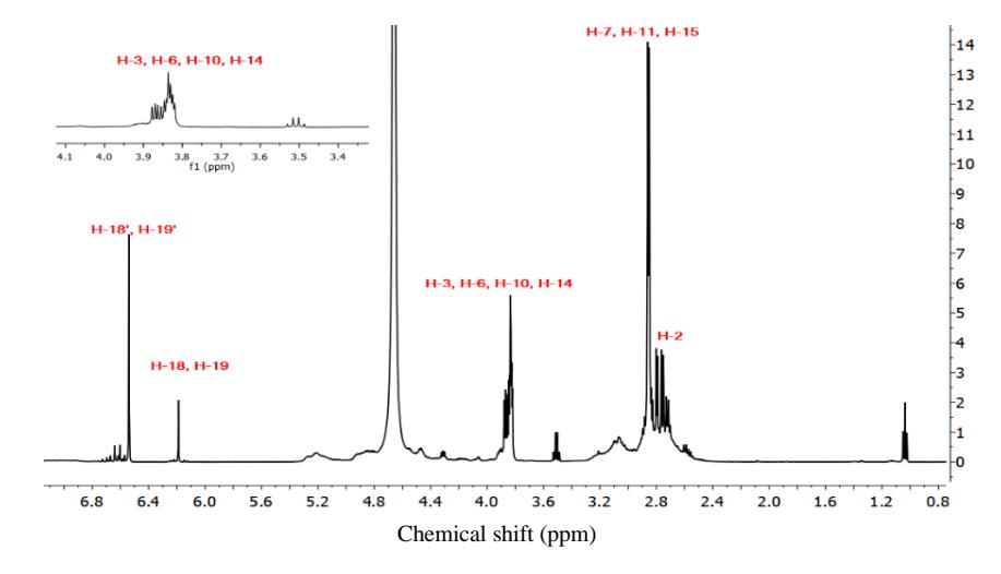
Figure 4 1H NMR spectra of OSI (in D2O).
The results of the 1H NMR spectra analysis confirmed three types of protons in the OSI compound, i.e. methanetriyl, single-bonded methane, and doublebonded methine protons at ending sides of the OSI chains. On the maleimide end groups, two protons could be in trans (H-18' and H-19') or cis (H-18 and H-19) configuration. Proton signals at 1.04 ppm and 3.52 ppm correspond to the presence of ethanol, which strongly interacted with OSI molecules. Furthermore, the types of carbons in this compound were determined by 13C NMR and DEPT 135 (Figures 5(a) and 5(b)).
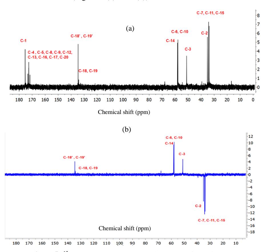
Figure 5 13C NMR (a) and DEPT 135 (b) spectra of OSI (in D2O).
It was clear that carbonyl carbons did not appear in a single signal, however, several carbon signals appeared at 171.6 to 175.4 ppm in the 13C NMR spectra due to differences in resonance frequency in the magnetic field between rings in the middle or main chain and rings in the end groups of the OSI structures. In addition, these quaternary carbons did not appear in the DEPT 135 spectra. One of the molecular structures of the OSI is composed of 5 repeating units; the complete chemical shifts of proton and carbon signals are shown in Figure 6 and Table 1 respectively.
\[\text{[rumus tidak dapat ditampilkan dengan baik — lihat PDF asli]}\]
Figure 6 One of the molecular structures of the synthesized OSI.
Table 1 <sup>1</sup>H NMR, <sup>13</sup>C NMR, and DEPT 135 chemical shifts of nuclei in OSI.
| Assignment from Fig. 6 | δH (ppm) | δC (ppm) | Assignment from Fig. 6 | δH (ppm) | \(\delta_{C}\left(ppm\right)\) |
|---|---|---|---|---|---|
| 1 | _ | 175.4 | 12 | _ | 172.7 |
| 2 | 2.71, 2.80 | 35.2 | 13 | _ | 172.6 |
| 3 | 3.87 | 51.2 | 14 | 3.83 | 58.2 |
| 4 | - | 173.4 | 15 | 2.76, 2.86 | 34.3 |
| 5 | _ | 172.6 | 16 | _ | 172.7 |
| 6 | 3.85 | 57.8 | 17 | _ | 171.6 |
| 7 | 2.76, 2.86 | 34.3 | 18 | 6.19 | 134.2 |
| 8 | _ | 172.7 | 19 | 6.19 | 134.2 |
| 9 | - | 172.6 | 18' | 6.54 | 134.6 |
| 10 | 3.85 | 57.8 | 19' | 6.54 | 134.6 |
| 11 | 2.76, 2.86 | 34.3 | 20 | _ | 171.6 |
3.3 Structure Characterization Using LC-MS
The numbers of repeating units on the oligomeric chain and their fractional distribution were analyzed by liquid chromatography-mass spectroscopy (LC-MS). The resulted chromatograms showed five major peaks of four major fractions of the synthesized compound within the retention time range from 1.17 to 2.53 minutes (Table 2). In this range, the average molecular weights of OSI were 461, 558, 654, and 752 g.mol<sup>-1</sup> respectively.
They were composed of four to seven repeating units in the formed closed ring structure. There are similar fractions that were eluted within the retention time range from 1.67 to 2.18 minutes owing to a lot of these fractions being present in the compound. Utilization of water-acetonitrile (polar solvents) as the mobile phase and formic acid as ionizing agent would initially elute the shorter or more polar chains of OSI fractions, causing a shorter retention time than other
fractions with longer chains. The mixture of all fractions was simultaneously evaluated in a corrosion inhibition test.
Table 2 Retention time and average molecular weight of each fraction oligosuccinimide derived from chromatogram and mass spectra data.
| Retention time (minute) | Fraction | Molecular weight (g.mol-1 ) |
|---|---|---|
| 1.17 | Tetramers | 461 |
| 1.27 | Pentamers | 558 |
| 1.67-2.18 | Hexamers | 654 |
| 2.53 | Heptamers | 752 |
3.4 Evaluations on Corrosion Inhibition Performance
The results from the corrosion inhibition analysis using EIS are displayed using Nyquist plots in Figure 7. These plots describe the relationship between the increase of semicircle/diameter sizes and the increment of the inhibitor concentration. Generally, corrosion inhibitor exhibited the size trends of semicircle/diameter from Nyquist curves increasing along with the increase of inhibitor concentration. This corresponds to an increase in the values of real (Zr) and imaginary (-Zi) impedances of the system. The irregular lines in the Nyquist plots were possibly caused by noise during the measurements.
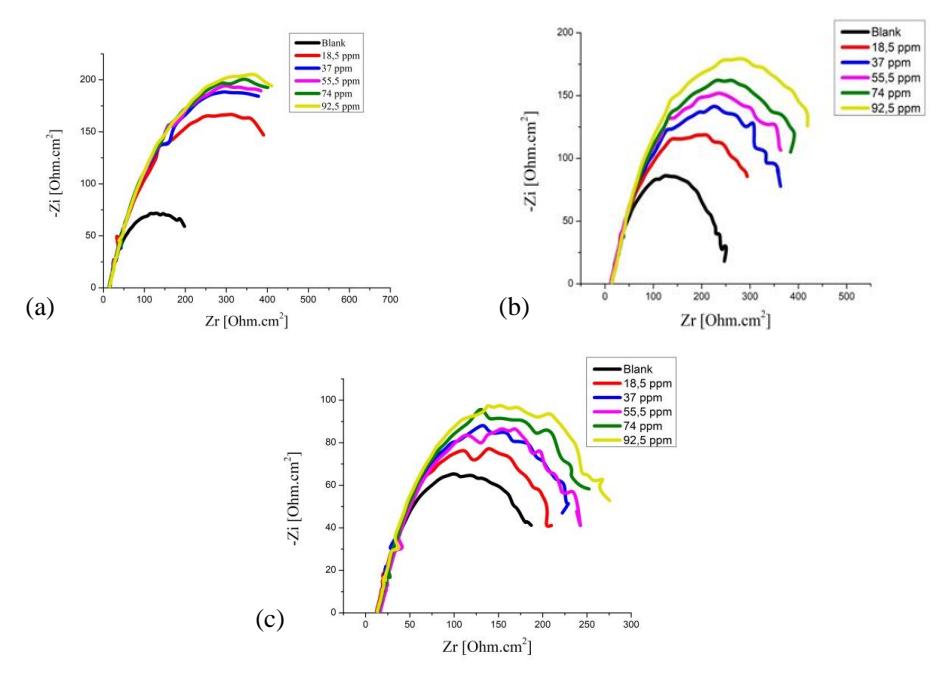
Figure 7 Nyquist plots for different concentrations of OSI at (a) 25 °C, (b) 35 °C, (c) 45 °C.
The values of Rct were obtained by subtracting the highest frequency of the real impedance from the lowest frequency one, as follows:
\[R_{ct} = Z_r \text{ (at low frequency)} - Z_r \text{ (at high frequency)}\] (5)
At low frequency, there are depressed peaks due to Zi being directly proportional with frequency based on Eq. (6):
\[Z_{i} = \frac{1}{2} \pi f C \tag{6}\] where f is the frequency and C is the electric capacitance. Various electrochemical parameters, i.e. corrosion potential (Ecorr), solution resistance (Rs), charge transfer resistance (Rct), electric double layer capacitance (Cdl), and efficiency of corrosion inhibition (IE), were analyzed using EIS for different concentrations and temperatures, as listed in Table 3.
Table 3 Parameters to evaluate OSI performance as corrosion inhibitor at several concentrations utilizing EIS at 25, 35, and 45 °C.
| Temp. | Concentration | Ecorr (mV | Rs | Rct | Cdl | IE |
|---|---|---|---|---|---|---|
| (°C) | (ppm) | Vs SCE) | (Ω.cm2 ) | (Ω.cm2 ) | (µF/cm2 ) | (%) |
| Blank | -700.1 | 13.99 | 252.8 | 281.9 | – | |
| 18.5 | -649.4 | 13.26 | 546.9 | 162.9 | 53.775 | |
| 37 | -648.6 | 13.27 | 637.1 | 158.1 | 60.320 | |
| 25 | 55.5 | -646.8 | 13.58 | 638.3 | 157.5 | 60.395 |
| 74 | -646.6 | 13.55 | 657.1 | 153.0 | 61.528 | |
| 92.5 | -642.9 | 14.41 | 678.0 | 148.3 | 62.714 | |
| Blank | -715.1 | 12.70 | 245.1 | 141.6 | – | |
| 18.5 | -671.8 | 13.07 | 342.5 | 126.7 | 28.467 | |
| 37 | -663.5 | 13.17 | 408.6 | 122.6 | 39.951 | |
| 35 | 55.5 | -675.6 | 13.14 | 442.1 | 112.1 | 44.570 |
| 74 | -653.1 | 16.02 | 464.2 | 102.2 | 47.198 | |
| 92.5 | -650.9 | 15.96 | 509.3 | 94.81 | 51.895 | |
| Blank | -720.1 | 13.50 | 201.2 | 121.7 | – | |
| 45 | 18.5 | -680.1 | 12.73 | 224.5 | 119.4 | 10.468 |
| 37 | -675.4 | 13.48 | 249.1 | 111.9 | 19.309 | |
| 55.5 | -670.1 | 17.14 | 250.5 | 103.3 | 20.143 | |
| 74 | -665.8 | 15.16 | 269.1 | 97.73 | 25.279 | |
| 92.5 | -665.7 | 13.74 | 292.6 | 88.67 | 31.164 |
The decrease of Cdl with the addition of inhibitor indicates a reduction in the local dielectric constant, followed by an increase in the thickness of the electrical double layer due to the adsorption of inhibitor and replacement of water molecules [21]. The value of Cdl is expressed by Helmholtz model as follows [3]:
\[C_{dl} = \frac{\varepsilon^{\circ}.\ \varepsilon.\ A}{d} \tag{7}\] where ε° is the permittivity of the air, ε is a dielectric constant of the solution, A is the effective surface area of the electrode, and d is thickness of the protective double layer. The results showed that inhibition efficiency reached 62.71% when the inhibitor concentration was 92.5 ppm. This corresponds to an increment of surface coverage (θ) to prevent direct contact between metal and corrosive substances [22].
The efficiency of corrosion inhibition can also be influenced by temperature [4]. EIS data showed that OSI had good capability as corrosion inhibitor, especially at 25 °C. However, the IE values decreased slowly after the temperature was raised. Higher temperatures can stimulate faster reactions to form corrosive ions (CO3 2− and H+ ) in solution and will accelerate the diffusion activity of substances from solution phase to the cathodic side of the metal surface for reduction reactions [23]. Moreover, the rate of electron transfer in parts of the metal to the solution will increase at higher temperature, also potentially releasing inhibitor molecules that are physically adsorbed on the surface back to the solution phase [24].
Subsequently, for potentiodynamic polarization, the efficiency of corrosion inhibition was measured based on the corrosion current density (Icorr) that was calculated by extrapolating the linear part of the anodic and cathodic Tafel slopes. These polarization curves are displayed in Figure 8.
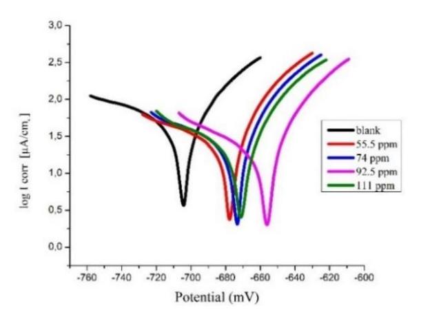
Figure 8 Polarization curve of OSI at 25 °C.
These curves show the cathodic Tafel slope (βc), which slightly changed compared to the anodic Tafel slope (βa) at all inhibitor concentrations. This clearly indicates that the addition of inhibitor did not significantly influence the proton-discharge reaction on the cathodic side, however, it was more likely to protect the mechanism of iron dissolution on the anodic side [25]. The relationship between the cathodic and the anodic Tafel slopes (mV/dec) related to this particular corrosion system, expressed by proportionality constant B, Icorr and corrosion rate (CR) in potentiodynamic polarization. These parameters were derived by using the Stern-Geary equation, as follows [26]:
\[B = \frac{\beta a \cdot \beta c}{2.3 (\beta a + \beta c)} \tag{8a}\]
\[I_{corr} = \frac{B}{R_{ct}} \tag{8b}\]
\[C_R = k.\,\mu_{eq}.\frac{I_{corr}}{d} \tag{8c}\] where k is constant, is the equivalent weight and d is density of carbon steel. This was also supported by the change in corrosion potential to more positive values after addition of inhibitor. Thus, the OSI predominantly acted as anodic inhibitor, however, the difference of its corrosion potential did not exceed 85 mV, thus OSI must be classified as a mixed inhibitor [25,27]. As a mixed inhibitor, OSI will be adsorbed on the metal surface by donating lone pair electrons or π-electrons to Fe atoms on the anodic side, slowing down metal dissolution and accepting electrons from 3d orbitals of the Fe atoms on the cathodic side to inhibit the hydrogen evolution reaction [28,29]. The complete results of the electrochemical parameters using potentiodynamic polarization are listed in Table 4.
Table 4 Results of corrosion inhibition analysis of OSI by potentiodynamic polarization at 25 °C.
| C (ppm) | Ecorr (mV) | βa (mV/dec) | βc (mV/dec) | Icorr (µA/cm2 ) | CR (µmPY) | IE (%) |
|---|---|---|---|---|---|---|
| Blank | -704.0 | 47.00 | -157.30 | 50.010 | 584.9 | – |
| 55.5 | -678.0 | 35.00 | -117.40 | 24.034 | 275.7 | 51.94 |
| 74 | -674.1 | 35.20 | -118.20 | 23.475 | 274.5 | 53.05 |
| 92.5 | -657.6 | 35.10 | -93.60 | 18.649 | 218.1 | 62.73 |
| 111 | -671.3 | 31.50 | -96.20 | 19.864 | 232.3 | 60.28 |
Table 4 displays several parameters, i.e. corrosion potentials, corrosion current density, and corrosion rate. The corrosion current density decreased by the presence of inhibitor followed by an increase of the inhibition efficiency when the concentration of OSI was raised to 92.5 ppm. These results are in accordance with the EIS measurements in Table 3, especially when the concentration of inhibitor was 92.5 ppm. The addition of more inhibitors did not significantly change the IE value. Instead, it decreased after the inhibitor concentration reached 111 ppm. One reason is the presence of attraction forces among adsorbed inhibitor molecules on the metal surface and others in the diffusion layer since the solution contains high concentrations of OSI.
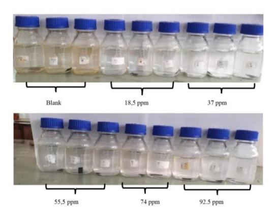
Figure 9 Visualization of bottles containing 1% (w/v) NaCl solution, saturated by CO2 gas without inhibitor and with inhibitor after the weight loss tests.
Consequently, the intermolecular attractions between the inhibitor molecules can desorb inhibitor molecules from the metal surface into the solution phase. Furthermore, the weight loss method was carried out to observe the influence of mechanical shock and the endurance of adsorbed inhibitor at a longer test time. Figure 9 shows the appearance of the bottles after weight loss testing. A slightly brown solution was visible in the three bottles without inhibitor, which indicates the amount of Fe ions in the solution phase. Meanwhile, the bottles with inhibitor displayed a clearer solution.
Figure 10 shows the results of this method, which had good agreement with the electrochemical method, indicating that there was no significant effect from mechanical shock and testing time toward the performance of the OSI as corrosion inhibitor because most of its molecules were still strongly adsorbed on the carbon steel surface at this temperature.
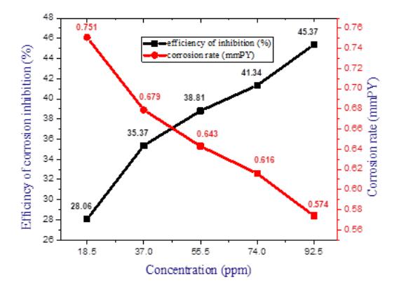
Figure 10 Relationship between inhibitor concentration and inhibition efficiency and corrosion rate using weight loss method at 35 °C for 48 hours.
3.5 Study of Adsorption Isotherm and Standard Gibbs Free Energy of Adsorption
The adsorption mechanism of the OSI on the carbon steel/solution interface was analyzed by several adsorption isotherms, i.e. the Langmuir, Temkin, and Freundlich isotherms. This analysis was based on the relation between the surface coverage values (θ) and the concentration of OSI which was tested graphically to obtain the best adsorption isotherm. The θ values were calculated from the efficiency of corrosion inhibition as follows:
\[\theta = \frac{\% IE}{100} \tag{9}\]
In this study, the Langmuir isotherm gave the best fit at 25 °C and 35 °C, as represented in Eq. (9). Strong correlations (R 2 = 0.9996 at 25 °C and 0.996 at 35 °C) confirm the validity of this approach. The linearity of Langmuir adsorption isotherm at 25 °C and 35 °C, is shown in Figure 11, which suggests that each inhibitor compound formed a monolayer on the carbon steel surface and there was no interaction between the adsorbed inhibitor molecules [30]. However, the linear regression coefficient of OSI at 45 °C had a smaller value (R 2 < 0.900) for the simplest form of the Langmuir adsorption isotherm.
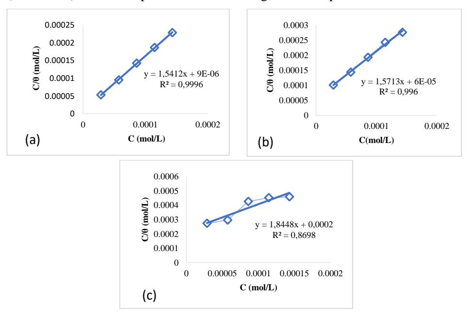
Figure 11 The linear relationship between the concentration of corrosion inhibitor (OSI), Cinh, and Cinh/θ, according to the simplest form of Langmuir the adsorption isotherm on Eq. (7) at (a) 25 °C, (b) 35 °C, (c) 45 °C, respectively.
Therefore, it was fitted by plotting \(\log(\theta/(1-\theta))\) to the logarithm of concentration (\(\log C_{inh}\)), which is the linear relationship of the modified Langmuir adsorption isotherm according to Eq. (11). Besides that, it was also fitted with other adsorption isotherm plots, such as the Freundlich and Temkin adsorption isotherms, as expressed in Eq. (12) and Eq. (13):
\[\frac{C}{\theta} = \frac{1}{K_{ads}} + C \tag{10}\]
\[\log\left(\frac{\theta}{1-\theta}\right) = \log K_{ads} + \log C \tag{11}\]
\[\log \theta = \log K_{ads} + \frac{1}{n} \log C \tag{12}\]
\[\theta = \frac{1}{f} \log K_{ads} + \frac{1}{f} \log C \tag{13}\] where C is the concentration of inhibitor (mol.L<sup>-1</sup>), \(K_{ads}\) is the equilibrium constant of adsorption, 1/n and 1/f are related to the adsorption intensity of adsorbate on metal [31]. The modified equation of Langmuir adsorption isotherm gave a linear regression coefficient above 0.9 (\(R^2 > 0.900\)) at 45 °C, (Figure 12), while the Freundlich isotherm gave the best fit at this temperature.
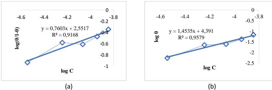
Figure 12 The linear relationship between \(\log(\theta/(1-\theta))\) and the logarithm of concentration of OSI (log \(C_{inh}\)), according to (a) the modified Langmuir adsorption isotherm and (b) the Freundlich adsorption isotherm at 45 °C.
The value of 1/n is more than 1 (1.4535). This indicates that the adsorption process was unfavorable at 45 °C [32]. Meanwhile, the type of adsorption was determined by calculating the standard Gibbs free energy of adsorption \(\Delta G_{ads}^o\), as follows:
\[\Delta G_{ads}^o = -RT \ln(55.5 \cdot K_{ads}) \tag{14}\] where R is the ideal gas constant (8.314 J.mol<sup>-1</sup>K<sup>-1</sup>), the value of 55.5 is the water concentration (mol.L<sup>-1</sup>) in solution, and T is temperature (K) [17].
The type of adsorption isotherm, concentration, surface coverage \((\theta)\), equilibrium constant \((K_{ads})\), and standard Gibbs free energy of adsorption of OSI
\((\Delta G_{ads}^o)\) are given in Table 5. Generally, the adsorption mechanism of OSI on a carbon steel surface obeys the Langmuir isotherm. Adsorption takes place via: (1) electrostatic attractions between charged molecules and charged metal; (2) interactions of lone pair electrons in inhibitor molecules with the metal; (3) interactions of \(\pi\)-electrons with the metal; and (4) a combination of all three processes [33]. All values of \(\Delta G_{ads}^o\) were negative and the values of \(K_{ads}\) were large. This showed that the adsorption of OSI molecules on the metal surface was a spontaneous process and had sufficient adsorption energy. The \(\Delta G_{ads}^o\) values were within the range of -33.14 to -38.73 kJ.mol<sup>-1</sup>, implying that the interactions of OSI molecules with the metal surface were characteristic of semi-physisorption. The interactions were more dominated by physisorption because the value was closer to -20 kJ.mol<sup>-1</sup> [34].
Table 5 Results of analysis type adsorption isotherm, equilibrium constant and standard Gibbs free energy of adsorption OSI within the range of 25-45 °C.
| T (°C) | Type of adsorption isotherm | C (ppm) | θ | Kads (L.mol-1) | \(\Delta G^{o}_{ads}\) (kJ.mol-1) | |
|---|---|---|---|---|---|---|
| 25 | Langmuir | 18.5 | 0.538 | 1.11 x 10⁵ | ||
| 37 | 0.603 | -38.73 | ||||
| 55.5 | 0.604 | |||||
| 74 | 0.615 | |||||
| 92.5 | 0.627 | |||||
| 18.5 | 0.285 | -35.18 | ||||
| 37 | 0.399 | |||||
| 35 | Langmuir | 55.5 | 0.446 | 1.67 x 10⁴ | ||
| 74 | 0.472 | |||||
| 92.5 | 0.519 | |||||
| Langmuir | 18.5 | 0.105 | 5 x 10³ | -33.14 | ||
| 37 | 0.193 | |||||
| 45 | 55.5 | 0.201 | ||||
| 74 | 0.253 | |||||
| 92.5 | 0.312 | |||||
| 45 | Freundlich | 18.5 | 0.105 | |||
| 37 | 0.193 | 2.46 x 10³ | ||||
| 55.5 | 0.201 | -37.35 | ||||
| 74 | 0.253 | |||||
| 92.5 | 0.312 | |||||
4 Conclusions
Oligosuccinimide was successfully synthesized by thermal condensation between maleic anhydride and ammonium carbonate as precursors. The synthesized oligomer compounds were hygroscopic and consisted of tetramers, pentamers, hexamers, and heptamers. The results of corrosion tests using EIS showed that OSI has capability as a corrosion inhibitor for carbon steel in 1%
(w/v) NaCl solution saturated by \(CO_2\) gas due to the increase of the charge transfer resistance. The highest inhibition efficiency (62.7%) after EIS analysis and potentiodynamic polarization was obtained at an OSI concentration of 92.5 ppm. The efficiency of corrosion inhibition increased along with an increase of inhibitor concentration but decreased when the temperature was raised. This inhibition efficiency is relatively low compared to other organic inhibitors, but can be sufficiently effective to protect carbon steel pipelines. The potentiodynamic polarization study revealed that OSI acts as a mixed inhibitor. The negative value of \(\Delta G_{ads}^o\) suggests that the OSI was adsorbed spontaneously. Its adsorption obeyed the Langmuir isotherm at 25 °C and 35 °C, whereas at 45 °C it obeyed the Freundlich isotherm. Oligosuccinimide molecules were strongly adsorbed on the surface of carbon steel, so there was no significant effect from mechanical shock and time toward the performance of OSI as corrosion inhibitor.
Acknowledgements
The first author received a scholarship from the Indonesia Endowment Fund for Education (LPDP). This research was also supported by the Department of Chemistry of Institut Teknologi Bandung and Central Laboratory of Universitas Padjadjaran Jatinangor.