
1 Introduction
This paper is devoted to the construction of explicit finite difference schemes to obtain an approximate solution for the following hyperbolic system in conservation-law form:
\[\partial_t u + \partial_x F(u, \gamma(x)) = \epsilon \partial_{xx} u, \qquad (x, t) \in \Omega := \mathbb{R} \times \mathbb{R}^+,\]
\[u(x, 0) = u_0(x), \qquad x \in \mathbb{R}, \qquad (1)\]
In Eq. (1), the unknown function = (,) has to be determined; 0 ∶ ℝ → ℝ is a prescribed function and is a small non-negative constant. The flux (, ()) in Eq. (1) has a possibly discontinuous spatial dependence through the coefficient (). Let us suppose that the function () is a piecewise smooth function with possibly a finite number of jump discontinuities. We further assume that () has only one point of discontinuity, which is located at = 0 for simplicity. This makes the line = 0 an interface for our problem.
A typical example of the flux functions that we will particularly consider has the following form:
\[F(u,\gamma(x)) = \gamma(x)f(u), \qquad \gamma(x) = \begin{cases} \gamma_L, x < 0, \\ \gamma_R, x > 0. \end{cases}\] (2)
Here, the function f is a smooth function and \(\gamma_{\alpha}\) for \(\alpha = L, R\) are two non-zero constants. Conservation laws with discontinuous flux function in x appear in various physical model problems in science and engineering, for example in the modeling of two-phase flow in porous media [1], in sedimentation problems [2-4] and in traffic flow on roads with varying conditions [5,6]. We also note that conservation laws with discontinuous flux can be modeled in different forms. For instance, the convective flux is in the form \(F(u, \gamma(x)) = \gamma(x) \cdot f(u) + (1 - \gamma(x)) \cdot g(u)\), where f, g are two given functions and \(\gamma\) is the Heaviside step function, see Andreianov, et al. [7] and Izadi [8-10]. Indeed, Eq. (1) is a special case of non-linear degenerate parabolic convection-diffusion model problems of the type
\[\partial_t u + \partial_x F(u, \gamma(x)) = \partial_{xx} A(u), \tag{3}\] where A is a given function. In Karlsen, et al. [11] the authors analyzed approximate solutions obtained based on an upwind difference method of the Engquist-Osher type for this type of problem. For the case of linear flux function f(u) = u in Eq. (2) and \(\epsilon = 0\), an immersed upwind interface method was introduced in Wen and Jin [12] to build the interface condition into the numerical flux. The Rung-Kutta discontinuous Galerkin method was developed in Okhovati and Izadi [13]. For an overview of some recent results devoted to problem Eq. (3), we refer the interested reader to Mishra [14] and the references therein. We note that if \(F(u, \gamma(x))\) is not dependent on x, then Eq. (1) reduces to the classical conservation law, which has a long tradition, see for example LeVeque [15]. The main difficulty in devising numerical schemes for classical (nonlinear) hyperbolic conservation laws is the presence of discontinuities in the solution, even though the initial condition \(u_0(x)\) and the flux function \(F(u, \gamma(x))\) are sufficiently smooth. Hence, one has to seek a solution for Eq. (1) in the weak sense. A function \(u \in L_{\infty}(\Omega)\) is called a weak solution of Eq. (1) if for all test functions \(\varphi \in C_0^{\infty}(\overline{\Omega})\) we have:
\[\int_{\Omega} (u \partial_t \varphi + G(u, \gamma(x)) \partial_x \varphi) dx dt = -\int_{\mathbb{R}} u_0(x) \varphi(x, 0) dx, \tag{4}\] where \(G(u, \gamma(x)) = F(u, \gamma(x)) - \epsilon \partial_x u\). Considering the flux function Eq. (2) it is not difficult to see that Eq. (4) is a weak formulation of the following problem. Denoting by \(g_{\alpha}(u) := \gamma_{\alpha} f(u) - \epsilon \partial_x u\), \(\alpha = L, R\), then in the weak sense u satisfies:
\[\partial_t u + \partial_x g_R(u) = 0, & x > 0, t > 0, \partial_t u + \partial_x g_L(u) = 0, & x < 0, t > 0, \nu(x,0) = u_0(x), & x \in \mathbb{R},\] (5)
and at the interface x = 0, solution u satisfies the Rankine-Hugoniot condition for zero-speed discontinuity, that is for almost all t > 0:
\[g_L(u(0^-,t)) = g_R(u(0^+,t)),\] (6)
where \(u(0^{\pm},t) = \lim_{s \to 0^{\pm}} u(x+s,t)\) are called the left and right traces. In addition, weak solutions are not uniquely determined by their initial data and an additional selection principle, the so-called entropy condition, is needed to single out physically meaningful weak solutions. At \(x \neq 0\), the most commonly used entropy condition is obtained by a Kružkov type entropy condition [16], which is derived from a regularization of the conservation laws. It is wellknown that for a problem Eq. (3) in which the coefficient \(\gamma(x)\) is discontinuous, the standard entropy condition (e.g. Kružkov) breaks down and a new entropy condition is needed to select a unique solution. Several existence and uniqueness results for the entropy solutions of Eq. (1) have been derived both from mathematical and physical considerations in a series of papers. In Karlsen, et al. [17], as a first step, the existence of a weak solution is proved by passing to the limit as \(\epsilon \downarrow 0\) in a suitable sequence \(\{u_{\epsilon}\}_{\epsilon>0}\) of smooth approximations solving problem Eq. (3) with flux \(\gamma(x)f(\cdot)\) replaced by \(\gamma_{\epsilon}(x)f(\cdot)\) and the diffusion function \(A(\cdot)\) replaced by \(A_{\epsilon}(\cdot)\), where \(\gamma_{\epsilon}(\cdot)\) is smooth and \(A'_{\epsilon}(\cdot)\)0. Karlsen, et al. [11] reconstructed approximate solutions with an upwind finite difference method and then showed that the limit of a converging sequence of difference approximations is a weak solution and satisfies a Kružkov type entropy inequality. For related work on other numerical methods for Eq. (3), see Andreianov, et al. [7] for a list of relevant references.
In this paper, we aimed to construct a simple numerical approximation method for Eq. (1) when convective flux Eq. (2) is utilized. The main focus was to investigate the applicability of the MacCormack scheme for convection-diffusion problems that have a discontinuous coefficient. In contrast to upwind schemes, which are only first-order accurate, in this work we propose the second-order MacCormack method, which is an explicit conservative finite difference scheme, to treat Eq. (1) numerically. The rest of this paper is organized as follows. In Section 1, some useful notations are introduced that will be used in the subsequent sections. Then we construct and study first-order accurate explicit upwind finite difference algorithms for one-dimensional convection-diffusion equations with discontinuous coefficients. This section may be seen as an extension of the upwind finite difference scheme proposed in Wen and Jin [12] in terms of flux functions. Section 3 is devoted to illustrating the explicit two-step MacCormack scheme applied to the model problem Eq.
(1). These schemes are then tested on several linear as well as non-linear problems in Section 4. We also justify the second-order accuracy of the MacCormack scheme throughout the course of numerical simulation. Finally, we draw some conclusions in Section 5.
2 First-Order Upwind Schemes
To proceed, we introduce some notations. Throughout this paper, the temporal and spatial discretization parameters in the proposed finite difference approximations will be denoted by \(\Delta t\) and \(\Delta x\), respectively, of the numerical schemes. Let the spatial domain \(\mathbb{R}\) be partitioned into uniform mesh elements \(I_j = [x_{j-\frac{1}{2}}, x_{j+\frac{1}{2}})\) with grid points \(x_{j-\frac{1}{2}} = j\Delta x\), \(j \in \mathbb{Z}\). Here, \(\Delta x = x_{j+\frac{1}{2}} - x_{j-\frac{1}{2}}\) is the mesh size. We will also set the midpoints of the intervals as \(x_j = \frac{1}{2}(x_{j-\frac{1}{2}} + x_{j+\frac{1}{2}})\), \(\forall j \in \mathbb{Z}\). Analogously, the time domain \(\mathbb{R}^+\) is partitioned into time strips \(I_n = [t_n, t_{n+1})\), where \(t_n = n\Delta t\) for \(n \in \mathbb{N} \cup \{0\}\), where \(\Delta t = t_{n+1} - t_n\) is the uniform time step. On the computational grid \((x_j, t_n)\) we use \(U_j^n\) to denote the computed finite difference solution to the exact solution \(u(x_j, t_n)\) of Eq. (1). We will also set
\[\mu = \frac{\Delta t}{\Delta x}\], \(I(v, w) = [\min\{v, w\}, \max\{v, w\}]\), \(\mu_{\alpha} = \gamma_{\alpha} \frac{\Delta t}{\Delta x}\), \(\alpha = L, R\).
The first-order upwind scheme plays an essential role in the development of second-order upwind methods. In fact, upwind schemes use concepts from characteristic theory to select the direction of spatial differencing. By simply ignoring the diffusion term \(\epsilon \partial_{xx} u\), Eq. (5) can be discretized using a first-order upwind scheme for the convective terms \(\gamma_{\alpha} f(u)\). To this end, let us discretize the initial data \(u_0(x)\). The initial condition \(u_0(x)\) is projected onto the space of piecewise constant functions by
\[U_{j}^{0} = \frac{1}{\Delta x} \int_{I_{j}} u_{0}(x) dx\], \(\forall j \in \mathbb{Z}\).
To proceed, let us have two (two-point) numerical flux functions: \(F_{\alpha} : \mathbb{R}^2 \to \mathbb{R}\) for \(\alpha = L, R\), which are locally Lipschitz continuous and satisfy the consistency property \(F_{\alpha}(u, u) = \gamma_{\alpha} f(u)\), \(\alpha = L, R\). Given \(U_j^n\) at time level \(t_n\), we calculate the discrete \(U_j^{n+1}\) via the following three-point numerical scheme:
\[U_{j-1}^{n+1} = U_{j-1}^{n} - \mu \left( F_{j,L}^{n} - F_{j-1,L}^{n} \right), \qquad j \le 0, \quad n \ge 0,\] (7)
\[U_j^{n+1} = U_j^n - \mu(F_{j+1,R}^n - F_{j,R}^n), \qquad j \ge 0, \quad n \ge 0,\] (8)
where \(F_{j,\alpha}^n = F_{\alpha}(U_{j-1}^n, U_j^n)\), \(\alpha = L, R\). Note that the coupling of the two finite difference schemes Eqs. (7-8) is carried out by evaluating \(F_{0,\alpha}^n = F_{\alpha}(U_{-1}^n, U_0^n)\),
\(\alpha = L, R\). In order to complete the definition of the presented method, we have to specify the numerical flux functions \(F_{\alpha}\), \(\alpha = L, R\). We utilize the standard upwind flux away from the interface. This implies that for \(j \neq 0\), the computation of \(F_{j,\alpha}^n\) is done by
\[F_{\alpha}(U,V) = \begin{cases} f_{\alpha}(U), & \text{if } \dot{s} \ge 0, \\ f_{\alpha}(V), & \text{if } \dot{s} < 0, \end{cases} \qquad \dot{s} = \begin{cases} \frac{f_{\alpha}(V) - f_{\alpha}(U)}{V - U}, & \text{if } U \ne V \\ \partial_{u} f_{\alpha}(U), & \text{if } U = V \end{cases}\](9)
where we have used \(f_{\alpha}(u) = \gamma_{\alpha} f(u)\) for \(\alpha = L, R\). In order to define the numerical coupling procedure, one needs to specify both fluxes \(F_{0,L}^n\) and \(F_{0,R}^n\) more precisely. For this purpose, depending on the sign of the derivative of \(f_{\alpha}\), the following cases are considered:
(1) If \(\partial_u f_\alpha(u) > 0\), \(\alpha = L\), R for all \(u \in I(U_j^n, U_{j+1}^n)\). In this case we only need to determine \(F_{0,R}^n\), which takes the form:
\[F_{0,R}^n = f_L(U_{-1}^n). (10)\]
For instance, in the case of linear flux \(f_{\alpha}(u) = \gamma_{\alpha} u\) with \(\gamma_{\alpha} > 0\), \(\alpha = L, R\), the numerical scheme Eqs. (7-8) can be rewritten as:
\[\begin{split} U_{j}^{n+1} &= (1 - \mu_{L}) U_{j}^{n} + \mu_{L} U_{j-1}^{n}, & \text{if} \quad j \leq -1, \\ U_{j}^{n+1} &= (1 - \mu_{L}) U_{j}^{n} + \mu_{R} U_{j-1}^{n}, & \text{if} \quad j = 0, \\ U_{j}^{n+1} &= (1 - \mu_{R}) U_{j}^{n} + \mu_{R} U_{j-1}^{n}, & \text{if} \quad j \geq 1. \end{split}\]
The parameters \(\mu_{\alpha}\), \(\alpha = L\), R are called the Courant-Friedrichs-Lewy numbers, or CFL numbers. They play a crucial role in determining the stability of the numerical scheme. Standard stability analysis dictates that these CFL numbers should be chosen such that \(0 < \mu_{\alpha} < 1\).
(2) If \(\partial_u f_\alpha(u) < 0\), \(\alpha = L, R\) for all \(u \in I(U_j^n, U_{j+1}^n)\). In this case it is sufficient to take \(F_{0,L}^n\) as
\[F_{0,L}^n = f_R(U_0^n). (11)\]
Again, utilizing the linear flux \(f_{\alpha}(u) = \gamma_{\alpha}u\) with \(\gamma_{\alpha} < 0\), \(\alpha = L\), R in Eqs. (7-8), after rearrangement one gets:
\[\begin{split} U_{j}^{n+1} &= (1+\mu_{L})U_{j}^{n} - \mu_{L}U_{j+1}^{n}, & \text{if} \quad j \leq -2, \\ U_{j}^{n+1} &= (1+\mu_{L})U_{j}^{n} - \mu_{R}U_{j+1}^{n}, & \text{if} \quad j = -1, \\ U_{j}^{n+1} &= (1+\mu_{R})U_{j}^{n} - \mu_{R}U_{j+1}^{n}, & \text{if} \quad j \geq 0. \end{split}\]
In the third case, we consider fluxes that have opposite signs.
(3) If \(\partial_u f_L(u) > 0\) and \(\partial_u f_R(u) < 0\) for all \(u \in I(U_j^n, U_{j+1}^n)\). In this situation, no extra requirement like Eq. (10) or Eq. (11) is needed for numerical treatment of the interface and the numerical flux defined in Eq. (9) is sufficient for computing \(U_{-1}^{n+1}\) and \(U_0^{n+1}\). If we consider the linear flux with \(\gamma_L > 0\) and \(\gamma_R < 0\) as in the two former cases, we get:
\[U_{j}^{n+1} = (1 - \mu_{L})U_{j}^{n} + \mu_{L}U_{j-1}^{n}, \quad \text{if} \quad j \leq -1, U_{j}^{n+1} = (1 + \mu_{R})U_{j}^{n} - \mu_{R}U_{j+1}^{n}, \quad \text{if} \quad j \geq 0.\]
Now, we can devise a finite difference approximation based on the upwind scheme mentioned above for Eq. (1) by discretizing the right-hand term \(\epsilon \partial_{xx} u\). For example, second- and fourth-order central difference approximations to \(\partial_{xx} u\) can be used. Introducing the following centered difference operators \(\delta_x^2 U_j = U_{j-1} - 2U_j + U_{j+1}\), one can approximate \(\partial_{xx} u\) at points \((x_j, t_n)\) as \(\frac{\delta^2 U_j^n}{\Delta x^2}\), which is obviously a second-order scheme. By means of the forward and backward difference operators
\[\Delta_x^- U_j = U_j - U_{j-1}, \qquad \Delta_x^+ U_j = U_{j+1} - U_j,\]
we modified the scheme Eqs. (7-8) for Eq. (1) as follows:
\[U_{j-1}^{n+1} = U_{j-1}^{n} - \mu \Delta_{x}^{-} F_{j,L}^{n} + \epsilon \lambda \delta_{x}^{2} U_{j}^{n}, \quad j \leq 0, \quad n \geq 0,\] (12)
\[U_{j}^{n+1} = U_{j}^{n} - \mu \Delta_{x}^{+} F_{j,R}^{n} + \epsilon \lambda \delta_{x}^{2} U_{j}^{n}, \qquad j \ge 0, \quad n \ge 0,\] (13)
where we have set \(\lambda \Delta x = \mu\). Note that since the upwind approximation Eqs.(7-8) is essentially a first-order scheme, the overall order of convergence cannot be improved upon, even if higher-order difference methods for other terms \(\partial_{xx}u\) and \(\partial_t u\) are employed.
3 Second-Order Schemes
The upwind approximation algorithms described in the last section are at most first-order accurate methods. These yield poor accuracy in regions where we have discontinuities or the exact solution is non-smooth. To overcome these problems, we utilize the idea of MacCormack [18] to formally upgrade the upwind scheme Eqs. (12-13) to second-order accuracy. This new scheme is obtained by correcting the first-order schemes; see Izadi [19], Kulmart and Pochai [20] for recent applications of the MacCormack schemes.
The standard algorithm based on the original MacCormack scheme consists of a two-stage procedure known as the predictor-corrector method. In fact, this method is a predictor-corrector version of the Lax-Wendroff scheme and is much easier to apply due to its Jacobian-free property. This explicit scheme can be presented for a single (classical) conservation law of the form \(\partial_t u + \partial_x H(u) = \epsilon \partial_{xx} u\) as follows:
\[U_{i}^{*} = U_{i}^{n} - \mu \Delta_{x}^{+} H_{i}^{n} + \epsilon \lambda \delta_{x}^{2} U_{i}^{n}, \qquad \text{(Predictor step)}\]
\[U_j^{**} = U_j^n - \mu \Delta_x^- H_j^{n,*} + \epsilon \lambda \delta_x^2 U_j^*. \quad \text{(Corrector step)}\]
Here, \(H_j^n\) and \(H_j^{n,*}\) are denoted by the flux H evaluated at \(U_j^n\) and \(U_j^*\) respectively. Hence, the solution at the next time level becomes:
\[U_j^{n+1} = \frac{1}{2} \left( U_j^* + U_j^{**} \right). \tag{16}\]
It should be stressed that the first-order spatial derivatives in Eqs. (14-15) are discretized with opposite one-sided finite differences in the corresponding predictor and corrector stages. The forward differencing operator is used in the predictor step and the backward differencing operator is used in the corrector step. However, applying these operators in these stages may be interchanged depending on the flux H, as we see in the case of our model problem. In order to write the MacCormack scheme in a conservative form and suitable for Eq. (1), we take the numerical fluxes \(H_{\alpha}\) as
\[H_{\alpha}(u,v) = \frac{1}{2} \left( f_{\alpha}(u) + f_{\alpha}(v) \right), \qquad \alpha = L, R\] (17)
Moreover, the average of u and v is defined as \(A(u,v) = \frac{1}{2}(u+v)\). In fact, by putting Eq. (14) into Eq. (15) followed by inserting the obtained result into Eq. (16) it can be written as conservative. Obtaining the predicted numerical values \(U_j^*\) in the first stage by upwind scheme Eqs. (12-13), the corrected numerical values \(U_i^{n+1}\) at the next time level are given by:
\[U_{j-1}^{n+1} = U_{j-1}^{n} - \mu \Delta_x^{\pm} H_{j,L}^{n,*} + \epsilon \lambda \delta_x^2 A_j^{n,*}, \quad j \le 0, \quad n \ge 0\] (18)
\[U_{j}^{n+1} = U_{j}^{n} - \mu \Delta_{x}^{\pm} H_{j,R}^{n,*} + \epsilon \lambda \delta_{x}^{2} A_{j}^{n,*}, \qquad j \ge 0, \quad n \ge 0,\] (19)
where \(H_{j,\alpha}^{n,*} = H_{\alpha}(U_{j-1}^n, U_j^*)\), \(A_j^{n,*} = A(U_j^n, U_j^*)\), \(\alpha = L, R\), and \(\Delta_x^{\pm}\) denotes either the forward or backward difference operator. As mentioned before, if for computing \(U_j^*\) in the range \(j \leq 0\) (\(j \geq 0\)) one uses \(\Delta_x^-\) (\(\Delta_x^+\)), which completely depends on \(f_{\alpha}\), then in Eqs. (18-19) we need to utilize a different one-sided operation that has the opposite sign. Utilizing the forward as well as the backward differences for space derivatives in calculating the average value of the time derivative in Eq. (16) is the main reason for the second-order accuracy. As an illustration, consider the linear flux functions \(f_{\alpha}(u) = \gamma_{\alpha}u\) for \(\alpha = L, R\) with \(\gamma_L > 0\), \(\gamma_R < 0\). Thus, the numerical schemes Eqs. (18-19) become:
\[U_{j}^{n+1} = U_{j}^{n} - \mu_{L} \Delta_{x}^{+} U_{j}^{*} + \epsilon \lambda \delta_{x}^{2} A_{j}^{n,*},\]
\[U_{j}^{*} = U_{j}^{n} - \mu_{L} \Delta_{x}^{-} U_{j}^{n} + \epsilon \lambda \delta_{x}^{2} U_{j}^{n},\]\nif \(j \leq -1\) and take the following form if \(j \geq 0\) \[U_{j}^{n+1} = U_{j}^{n} - \mu_{R} \Delta_{x}^{-} U_{j}^{*} + \epsilon \lambda \delta_{x}^{2} A_{j}^{n,*},\] \[U_{j}^{*} = U_{j}^{n} - \mu_{R} \Delta_{x}^{+} U_{j}^{n} + \epsilon \lambda \delta_{x}^{2} U_{j}^{n}.\]
4 Numerical Tests
We now investigate the performance of the MacCormack scheme applied to problem Eq. (1). We consider spatial domain [-1,1] by dividing it into N subintervals with \(N=2^s\), \(s=4,5,\cdots,10\). The time interval [0,T] is partitioned into \(nt=\lceil \frac{T}{\Delta t} \rceil\) small time-steps. To check the accuracy of the presented methods, the relative \(L_1, L_2\) and \(L_\infty\) error norms between the exact solution \(u_e\) and the numerical solution \(u_h\) are given by the following definitions: \(E(h,p)=\frac{\|u_h(T_1)-u_e(T_2)\|_p}{\|u_e(T_2)\|_p}\), \(p=1,2,\infty\). Here, \(0< T_1,T_2 \le T\). Note that for non-linear flux, the values of \(T_1\) and \(T_2\) may not be exactly equal, but \(|T_1-T_2|<\Delta t\). The rate of convergence is calculated using the formula \(\log_2\frac{E(h,p)}{E(\frac{h}{2},p)}\) for \(p=1,2,\infty\).
4.1 Linear case
In a linear case, we consider the linear flux \(f_{\alpha}(u) = \gamma_{\alpha}u\). Using the Fourier method, we can show that applying the MacCormack scheme to \(\partial_t u + \partial_x f_{\alpha}(u) = \epsilon \partial_{xx} u\) is stable under the CFL condition \(\left(\frac{|\gamma_{\alpha}|}{\Delta x} + \frac{2\epsilon}{(\Delta x)^2}\right) \Delta t \leq 1\), see [21]. By setting \(\gamma_{\max} = \max\{|\gamma_L|, |\gamma_R|\}\) to ensure stability, time step \(\Delta t\) is chosen as \(\Delta t = C_{cfl} \cdot \frac{(\Delta x)^2}{\Delta x \, \gamma_{\max} + 2\epsilon}\), where \(\Delta x = \frac{2}{N}\). Here \(C_{cfl}\) is an appropriate safety factor to keep the CFL below the stability limit. In this case, the final time T = 0.5 is used for the computations. We also set \(C_{cfl} = 0.025\).
Example 4.1 We first consider the model problem Eq. (1) with \(\gamma_L = 0.02\) and \(\gamma_R = -0.04\) and take \(u_0(x)\) with discontinuities at \(\pm \frac{1}{4}\), \(\pm \frac{3}{4}\) defined as
\[u(x,0) = 1\], for \(|x| \le \frac{1}{4}\),
\(u(x,0) = \frac{1}{2}\), for \(\frac{1}{4} < |x| \le \frac{3}{4}\),
\(u(x,0) = 0\), otherwise.
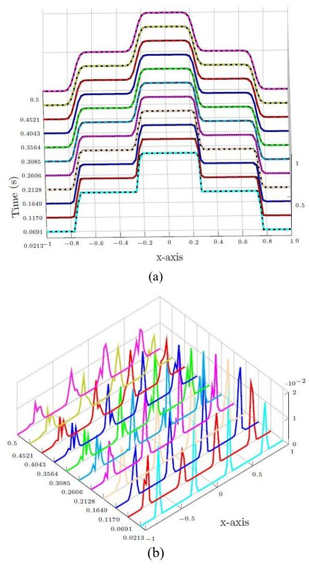
Figure 1 (a) Numerical and exact solutions and (b) the corresponding absolute errors of Example 4.1 at times = 4∆, 13∆, 22∆, . . . ,85∆, 94∆.
First, for a fixed = 80, visualizing the numerical solutions together with the exact solutions at times = 4∆, 13∆, 22∆, . . . ,85∆, 94∆ in Figure 1(a). Moreover, the corresponding absolute errors are depicted in Figure 1(b). In all plots we have used = 0.001.
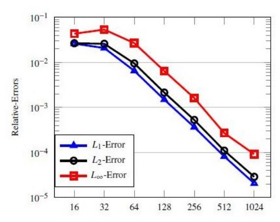
Figure 2 Relative 1 , 2 and ∞ errors evaluated at time = for different .
It can be seen from Figure 1(a) that the numerical results are in good agreement with the analytical results. However, some inefficiencies are observed in the vicinity of discontinuities. For this example we also investigated the behavior of relative errors with respect to in three different norms, 1, 2 and ∞, as shown in Figure 2. These results were evaluated at time = . In the Table 1 we report the corresponding convergence rates for different . As expected, the best results were obtained in the 1 norm. Finally, we investigated the impact of different values of viscosity ϵ on the MacCormack scheme. We took = 0.1,0.01,0.001,0.0001 and = 0. The numerical solutions at time = for these values of viscosity and for the number of spatial grid points = 80 are presented in Figure 3. As expected, the approximate solutions for different ϵ continuously tend to the solution corresponding to = 0. Note that when selecting less than 0.00001, almost the same number of time-steps ≈ 32 were obtained and therefore distinguishing between different solutions may be difficult.
Table 1 Relative 1 , 2 and ∞ convergence rates evaluated at time = for different .
| N | L1-order | L2-order | L∞-order |
|---|---|---|---|
| 16 | - | - | - |
| 32 | 0.32 | 0.04 | -0.31 |
| 64 | 1.68 | 1.45 | 1.00 |
| 128 | 2.12 | 2.15 | 2.01 |
| 256 | 2.03 | 2.02 | 2.00 |
| 512 | 2.16 | 2.27 | 2.59 |
| 1024 | 1.99 | 1.93 | 1.56 |
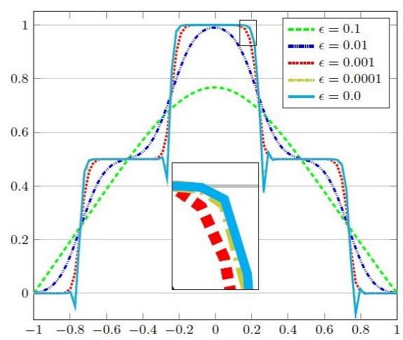
Figure 3 Numerical solutions for Example 4.1 evaluated at time t = T with \(\epsilon = 0.1, 0.01, 0.001, 0.0001\) and \(\epsilon = 0\).
Example 4.2 In this example, we again consider a linear case using wave speeds \(a_L = 0.04\) and \(a_R = 0.07\) with the same signs and a continuous initial data, \(u_0(x) = \sin^7(3\pi x)\). In this case, in view of the flux coupling condition, the exact solution for \(\epsilon = 0\) is obtained by following the characteristics lines. Having positive wave speeds, it becomes
\[u(x,t) = u_0(x - \gamma_L t), x < 0,\]
\[u(x,t) = \frac{\gamma_L}{\gamma_R} u_0 \left( \frac{\gamma_L}{\gamma_R} x - \gamma_L t \right), 0 < x < \gamma_R t,\]
\[u(x,t) = u_0(x - \gamma_R t), x > \gamma_R t.\]
In the second experiment, we take N=256 and \(\epsilon=0\). A snapshot of the numerical solution at the final time instant t=T is displayed in Figure 4. The exact solution is shown by the solid line. A comparison of the results obtained by the presented scheme, i.e. the MacCormack method, and those obtained by upwind difference approximation scheme Eqs. (7-8) is shown in Figure 4. Referring to Figure 4, it can obviously be seen that the MacCormack scheme outperformed the upwind method, especially near the corners.
In Table 1 we report the convergence rates of both methods in the relative \(L_1\), \(L_2\) and \(L_{\infty}\) norms. In the last column of Table 1, we also report the CPU times in seconds (sec) needed by the upwind and MacCormack schemes using N=256,512,1024. As expected, the time required by the MacCormack method was about two-fold compared to the upwind scheme.
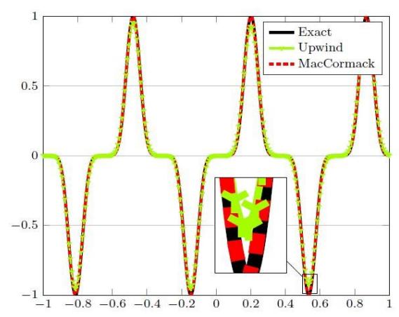
Figure 4 Numerical and exact solutions for Example 4.2 at times t = T for N = 256.
The results shown in Table 1 indicate that achieving first-order accuracy is possible with the upwind method while the corresponding order is two with the MacCormack scheme, especially when the number of cells is increased. Therefore, applying these methods for problems with discontinuities in an appropriate way can also lead to the same order of accuracy for continuous problems.
Table 2 Relative \(L_1\), \(L_2\) and \(L_\infty\) Convergence Rates for Example 4.2 Evaluated at Time t = T
| • | \(L_{I}\text{-}\mathrm{order}\) | L2-order | \(L_\infty\)-order | CPU time (sec) | ||||
|---|---|---|---|---|---|---|---|---|
| N - | Upwind | Mac- Cormack | Upwind | Mac- Cormack | Upwind | Mac- Cormack | Upwind | Mac- Cormack |
| 16 | - | - | - | - | - | - | - | - |
| 32 | 0.53 | 0.79 | 0.59 | 0.73 | 0.43 | 0.59 | ||
| 64 | 0.79 | 1.62 | 0.83 | 1.60 | 0.68 | 1.34 | ||
| 128 | 0.89 | 1.88 | 0.85 | 1.86 | 0.80 | 1.79 | ||
| 256 | 0.94 | 1.98 | 0.91 | 1.97 | 0.88 | 1.96 | 0.0028 | 0.0069 |
| 512 | 0.97 | 2.00 | 0.95 | 2.00 | 0.94 | 1.99 | 0.0118 | 0.0261 |
| 1024 | 0.98 | 1.99 | 0.98 | 2.00 | 0.97 | 2.00 | 0.0506 | 0.1247 |
4.2 Nonlinear case
To further demonstrate the accuracy of the proposed predictor-corrector scheme, we consider Eq. (1) with non-linear flux. We take \(f(u) = \frac{u^2}{2}\), which is known as the Burgers flux. For nonlinear problems, obtaining a simple stability criterion with the MacCormack scheme applied to them is not an easy task. In particular, stability analysis of the viscous Burgers equations does not lead to an exact and simple expression. Following Hoffmann [21], we also consider the following stability requirements for + () = , which are mainly obtained by numerical experimentations:
\[\left( |\gamma_{\alpha}u| \frac{\Delta t}{\Delta x} + 2\epsilon \frac{\Delta t}{(\Delta x)^2} \right) \le 1, \quad \text{or} \quad \Delta t \le \left\{ \frac{\Delta x}{|\gamma_{\alpha}u|}, \frac{(\Delta x)^2}{2\epsilon} \right\}.\]
Note that the stability condition will change during the computations. Thus, the time and space step sizes must be automatically adapted at each time level. For this purpose, time step ∆ should be chosen such that
\[\Delta t = C_{cfl} \cdot \frac{(\Delta x)^2}{\sup_j \left| \gamma_\alpha U_j^n \middle| \Delta x + 2\epsilon \right|}\]
In the computations below, we use fl = 0.1 and the final time is = 0.75.
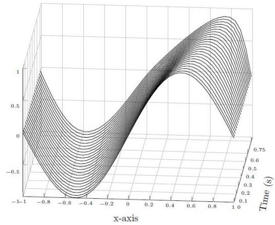
Figure 5 Numerical solutions for Example 4.3 after 1,5,10, . . . ,110,115 time levels with = 0.01.
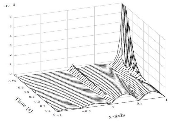
Figure 6 Absolute errors for Example 4.3 after 1,2,4, . . . ,56,58 time levels with = 0.
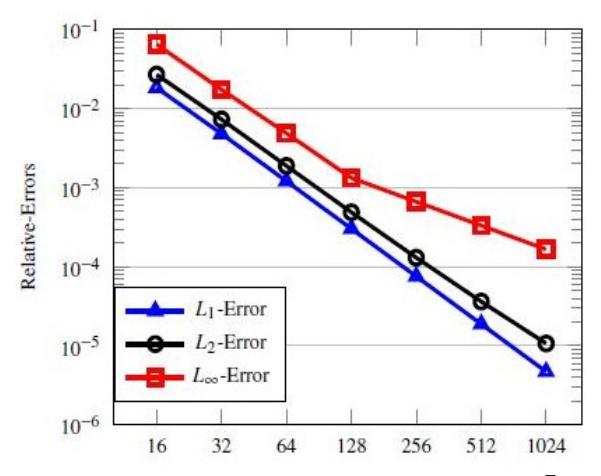
Figure 7 Relative \(L_1, L_2\) and \(L_{\infty}\)-errors evaluated at time \(t = \lfloor \frac{T}{2} \rfloor\) for different N.
Example 4.3 We first solve the non-linear model problem Eq. (1) with \(\gamma_L = 0.1\) and \(\gamma_R = 0.4\) and the initial data for this problem is \(u(x, 0) = \sin(\pi x)\).
For this problem, the viscosity is taken to be \(\epsilon = 0.01\) and N = 40. The numerical solutions after 1,5,10,...,110,115, time steps are visualized in Figure 5. When \(\epsilon = 0\), one can compute the exact solution of Eq. (1) with Burgers fluxes. Given the (smooth) initial data, the exact solution is obtained by the method of characteristics. Of course, these solutions are valid prior to the collision of the characteristics and after the appearance of shocks the solution achieved by this method may be considered invalid. It is not difficult to show that for the flux functions \(f_{\alpha}(u) = \gamma_{\alpha} \frac{u^2}{2}\) for \(\alpha = L, R\), the breaking times (of characteristics) are determined by
\[T_{\alpha} = \min_{x \in \mathbb{R}} \left| -\frac{1}{\gamma_{\alpha} u_0(x)} \right|, \qquad \alpha = L, R.\]
For our example these times are evaluated as \(T_L = \frac{10}{\pi} \approx 3.18\) and \(T_R = \frac{10}{4\pi} \approx 0.80\). For the coupling of two hyperbolic conservation laws, we calculate the absolute errors at various time levels as in Figure 5; the results can be seen in Figure 6. As is clear from this plot, some loss in efficiency will appear as time evolves towards the shock propagation time, \(t = T_R\). However, in the smooth regions and even near the interface x = 0 the errors are negligible compared to the shock region.
The exact knowledge of the solution allows us to draw precise conclusions about the accuracy and the order of the proposed method. Analogue to linear cases, we also justified the theoretical order of convergence of the MacCormack scheme by numerical results. We computed the \(L_1, L_2\) and \(L_\infty\) errors for different values of shown in Figure 7. The corresponding orders of convergence were also obtained through a grid-refinement study of the MacCormack scheme, as shown in the Table 3. Note that these results were computed at time = ⌊ 2 ⌋.
Table 3 Relative 1 , 2 and ∞ convergence rates evaluated at time = ⌊ 2 ⌋ for different .
| N | L1-order | L2-order | L∞-order |
|---|---|---|---|
| 16 | - | - | - |
| 32 | 1.94 | 1.88 | 1.90 |
| 64 | 1.99 | 1.95 | 1.84 |
| 128 | 2.00 | 1.95 | 1.88 |
| 256 | 2.00 | 1.91 | 1.00 |
| 512 | 2.00 | 1.84 | 1.00 |
| 1024 | 2.00 | 1.76 | 1.00 |
5 Conclusions
In this paper, a class of finite-difference schemes for convection-diffusion problems with discontinuous coefficient arising from the modeling of many real-world phenomena was described; the convective numerical flux is the upwind flux in these calculations. The original MacCormack scheme was modified based on the upwind methods to treat these problems numerically. First- and second-order upwind methods were compared using explicit code in both linear and non-linear model problems. One can easily confirm that the MacCormack method simulates the shock, which in the non-linear Example 4.3 corresponds to = 0, better than the first-order accurate schemes.