
1 Introduction
Mathematical models are applied widely to solve infectious disease problems [1-7]. One such disease is dengue fever, which is difficult to eradicate. Recently, a number of researchers have studied the spread of dengue, for example, Wagner, et al. [8], Windarto, et al. [9], and Zhu, et al. [10]. A type of mathematical model that is suitable for simulation of the spreading of dengue fever is the SIR-type model [11-14]. In SIR-type models, the total population is subdivided into three groups, namely, S (susceptible), I (infected), and R (recovered). Mathematical methods have also been employed to solve the dengue fever disease problem based on geographical area. Fakhruddin, et al. [15] used daily data of infection in Bandung to model the problem. Ramadhan, et al. [16] used the homotopy perturbation method (HPM) to simulate the disease's transmission in Makassar. Rangkuti, et al. [17] used HPM and the variational iteration method (VIM) to solve the dengue spreading problem in South Sulawesi. Other studies are also available in the literature based on the characteristics of local problems [18-21].
The SIR model of dengue fever is generally given in the form of a system of ordinary differential equations. An exact solution for the general case of the SIR model is not available. The SIR model can be solved using approximate approaches either numerically or analytically. Numerical approximate methods can solve the model for large domains (long time periods) but cannot provide explicit solutions. Analytical approximate methods may not be accurate for long time periods but can provide explicit functions as approximate solutions and are very accurate around the initial conditions of the problem.
This study focused on solving the SIR model of the spread of dengue fever in the case of South Sulawesi, as its prevalence in this province of Indonesia is relatively high [17]. When explicit functions are desired as solutions to the model, analytical approaches are powerful. We recall the work of Rangkuti, et al. [17] as well as that of Side and Noorani [22].
This paper makes, four contributions, which were the research goals. Firstly, in order to solve the SIR model of dengue fever transmission, we provide the successive approximation method (SAM). Secondly, we show that SAM is identical with Rangkuti's variational iteration method (RVIM) from Rangkuti, et al. [17]. Thirdly, we propose a modification of RVIM. Fourthly, we show that the modification of RVIM is more accurate. We call the modified method the improved Rangkuti's variational iteration method (IRVIM).
The rest of this paper is organized as follows. In Section 2, we describe the problem under consideration. We achieve our first three contributions in Section 3. Then, we achieve our fourth contribution in Section 4. We provide the conclusion of the paper in Section 5.
2 Problem Description
This section recalls the SIR model of the spread of dengue fever from the work of Side and Noorani [22]. Side and Noorani [22] studied the spread of dengue fever in the province of South Sulawesi (Indonesia) and in the state of Selangor (Malaysia) with a Susceptible-Infected-Recovered (SIR) model. Their original SIR model consisted of three compartments for the host (human) and two compartments for the vector (mosquitoes), which are given by the following system of five equations:
\[\frac{dS_h(t)}{dt} = \mu_h N_h - \frac{\beta_h b}{N_h} I_v(t) S_h(t) - \mu_h S_h(t), \tag{1}\]
\[\frac{dI_h(t)}{dt} = \frac{\beta_h b}{N_h} I_v(t) S_h(t) - (\mu_h + \gamma_h) I_h(t), \tag{2}\]
\[\frac{dR_h(t)}{dt} = \gamma_h I_h(t) - \mu_h R_h(t), \tag{3}\]
\[\frac{dS_{v}(t)}{dt} = \mu_{v} N_{v} - \frac{\beta_{v} b}{N_{h}} I_{h}(t) S_{v}(t) - \mu_{v} S_{v}(t), \tag{4}\]
\[\frac{dI_v(t)}{dt} = \frac{\beta_v b}{N_h} I_h(t) S_v(t) - \mu_v I_v(t), \tag{5}\]
A flowchart of this model is shown in Figure 1. Here, subscript h stands for the host and subscript v stands for the vector. \(S_h\) denotes the susceptible group of the host, \(I_h\) represents the infected group of the host, \(R_h\) denotes the recovered group of the host, \(S_v\) denotes the susceptible group of the vector, and \(I_v\) denotes the infected group of the vector. All involved parameters, \(\beta_h\), b, \(\mu_h\), \(\gamma_h\), \(\mu_v\), and \(\beta_v\), are nonnegative.
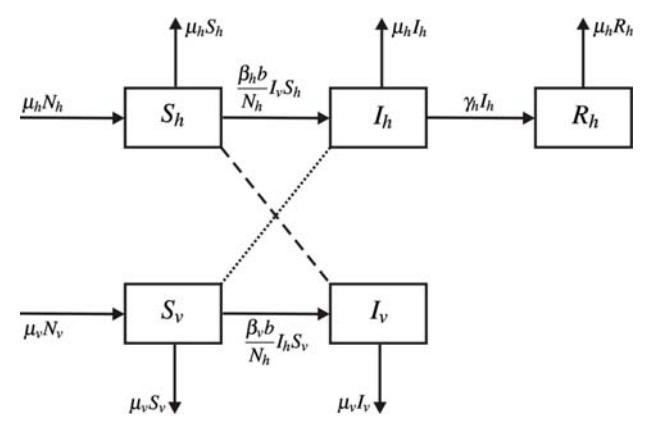
Figure 1 Flowchart of the SIR model of the spread of dengue fever, where the dotted line represents that there is interaction between \(I_h\) and \(S_v\), and the dashed line represents that there is interaction between \(S_h\) and \(I_v\).
Given that
\[S_h + I_h + R_h = N_h, \tag{6}\]
\[S_v + I_v = N_v, \tag{7}\]
we express the system of Eqs. (1-5) as a system of three equations:
\[\frac{dS_{h}(t)}{dt} = \mu_{h} N_{h} - \frac{\beta_{h} b}{N_{h}} I_{v}(t) S_{h}(t) - \mu_{h} S_{h}(t), \tag{8}\]
\[\frac{dI_h(t)}{dt} = \frac{\beta_h b}{N_h} I_v(t) S_h(t) - (\mu_h + \gamma_h) I_h(t), \tag{9}\]
\[\frac{dI_v(t)}{dt} = \frac{\beta_v b}{N_h} I_h(t) S_v(t) - \mu_v I_v(t). \tag{10}\]
We denote \(A = \mu_v N_v\). Using the new system of Eqs. (8-10), \(R_h\) and \(S_v\) can be obtained from the relations
\[R_h = N_h - S_h - I_h, \tag{11}\]
\[S_v = \frac{A}{\mu_v} - I_v. \tag{12}\]
We note that the total number \(N_h\) of the host population and the total number \(N_v\) of the vector population are constants, which can be verified by adding Eqs. (1-3), resulting in
\[\frac{dN_h}{dt} = \frac{dS_h}{dt} + \frac{dI_h}{dt} + \frac{dR_h}{dt} = 0 \tag{13}\] and adding Eqs. (4-5) leading to
\[\frac{dN_v}{dt} = \frac{dS_v}{dt} + \frac{dI_v}{dt} = 0. \tag{14}\]
Introducing new variables
\[x = \frac{S_h}{N_h}, \quad y = \frac{I_h}{N_h}, \quad u = \frac{R_h}{N_h}\] (15)
\[w = \frac{S_v}{N_v}, \quad z = \frac{I_v}{N_v},\tag{16}\]
we rewrite the system of Eqs. (8-10) as the normalized system of equations
\[\frac{dx(t)}{dt} = \mu(1 - x(t)) - \alpha x(t)z(t), \tag{17}\]
\[\frac{dy(t)}{dt} = \alpha x(t)z(t) - \beta y(t), \tag{18}\]
\[\frac{dz(t)}{dt} = \gamma (1 - z(t)) y(t) - \eta z(t), \tag{19}\] where
\[\mu = \mu_h\], \(\alpha = \frac{\beta_h b A}{\mu_v N_h}\), \(\beta = \gamma_h + \mu_h\), \(\gamma = \beta_v b\), \(\eta = \mu_v\). (20)
With this normalized system of Eqs. (17-19) we have x + y + u = 1 and w + z = 1. Furthermore, solutions to the original system of Eqs. (1-5) can be obtained from the solutions to the system of Eqs. (17-19), which is a simpler system. Hence, we concentrate on solving the system of Eqs. (17-19) with given initial conditions at t = 0 as
\[x(0) = x_0, y(0) = y_0, z(0) = z_0.\] (21)
We refer to Esteva and Vargas [23] and Yaacob [24] for the qualitative analysis and the qualitative solution to the system of Eqs. (1-5) and the system of Eqs. (17-19).
3 Successive Approximation and Variational Iteration Methods
This section contains four subsections. In Subsection 3.1, we recall RVIM proposed by Rangkuti, et al. [17], which is the basis of our work. To achieve the first goal of this paper, in Subsection 3.2 we provide SAM for solving the system of Eqs. (17-19). To achieve the second goal of this paper, in Subsection 3.3 we show that SAM is actually the same as RVIM for solving the system of Eqs. (17-19). To achieve the third goal of this paper, in Subsection 3.4 we propose a modification of RVIM for solving the system of Eqs. (17-19) to get more accurate solutions. The fourth goal of this paper will be achieved in the Results and Discussion section (Section 4).
3.1 Rangkuti's Variational Iteration Method (RVIM)
Here we recall the derivation of RVIM by Rangkuti, et al. [17]. RVIM is the basis of our work in this paper. The correction functionals for Eqs. (17-19) with initial conditions in Eq. (21) are:
\[x_{n+1}(t) = x_n(t) + \int_0^t \lambda_1(\tau) \left[ \frac{dx_n}{d\tau} - \mu \left( 1 - x_n(\tau) \right) + \alpha \tilde{x}_n(\tau) \tilde{z}_n(\tau) \right] d\tau, \tag{22}\]
\[y_{n+1}(t) = y_n(t) + \int_0^t \lambda_2(\tau) \left[ \frac{dy_n}{d\tau} - \alpha \tilde{x}_n(\tau) \tilde{z}_n(\tau) + \beta y_n(\tau) \right] d\tau, \quad (23)\]
\[z_{n+1}(t) = z_n(t) + \int_0^t \lambda_3(\tau) \left[ \frac{dz_n}{d\tau} - \gamma \tilde{y}_n(\tau) + \gamma \tilde{y}_n(\tau) \tilde{z}_n(\tau) + \eta z_n(\tau) \right] d\tau.\] (24)
Here \(\tilde{x}_n\), \(\tilde{y}_n\), and \(\tilde{z}_n\) are restricted variations meaning that \(\tilde{x}_n\), \(\tilde{y}_n\), and \(\tilde{z}_n\) behave as constants, so \(\delta \tilde{x}_n = 0\), \(\delta \tilde{y}_n = 0\), and \(\delta \tilde{z}_n = 0\); and \(\lambda_1(\tau)\), \(\lambda_2(\tau)\), \(\lambda_3(\tau)\) are Lagrange multipliers, which via the variational theory can be obtained optimally.
Taking the variations of Eqs. (22-24), we have:
\[\delta x_{n+1}(t) = \delta x_n(t) + \delta \int_0^t \lambda_1(\tau) \left[ \frac{dx_n}{d\tau} - \mu \left( 1 - x_n(\tau) \right) + \alpha \tilde{x}_n(\tau) \tilde{z}_n(\tau) \right] d\tau, \tag{25}\]
\[\delta y_{n+1}(t) = \delta y_n(t) + \delta \int_0^t \lambda_2(\tau) \left[ \frac{dy_n}{d\tau} - \alpha \tilde{x}_n(\tau) \tilde{z}_n(\tau) + \beta y_n(\tau) \right] d\tau, \tag{26}\]
\[\delta z_{n+1}(t) = \delta z_n(t) + \delta \int_0^t \lambda_3(\tau) \left[ \frac{dz_n}{d\tau} - \gamma \tilde{y}_n(\tau) + \gamma \tilde{y}_n(\tau) \tilde{z}_n(\tau) + \eta z_n(\tau) \right] d\tau. \tag{27}\]
After some operations, we obtain:
\[\delta x_{n+1}(t) = \delta \left[ \left( 1 + \lambda_1(t) \right) x_n(t) \right] - \delta \int_0^t \left[ \lambda_1'(\tau) - \mu \lambda_1(\tau) \right] x_n(\tau) d\tau, (28)\]
\[\delta y_{n+1}(t) = \delta \left[ \left( 1 + \lambda_2(t) \right) y_n(t) \right] - \delta \int_0^t \left[ \lambda_2'(\tau) - \beta \lambda_2(\tau) \right] y_n(\tau) d\tau, \tag{29}\]
\[\delta z_{n+1}(t) = \delta \left[ \left( 1 + \lambda_3(t) \right) z_n(t) \right] - \delta \int_0^t \left[ \lambda_3'(\tau) - \eta \lambda_3(\tau) \right] z_n(\tau) d\tau. \tag{30}\]
Then, the stationary conditions are:
\[(1 + \lambda_1(t))|_{\tau=t} = 0, \quad (\lambda'_1(\tau) - \mu \lambda_1(\tau))|_{\tau=t} = 0,\] (31)
\[(1 + \lambda_2(t))|_{\tau=t} = 0, \quad (\lambda'_2(\tau) - \beta \lambda_2(\tau))|_{\tau=t} = 0,\] (32)
\[(1 + \lambda_3(t))|_{\tau=t} = 0, \quad (\lambda_3'(\tau) - \eta \lambda_3(\tau))|_{\tau=t} = 0.\] (33)
Solving the stationary conditions in Eqs. (31-33), we obtain the Lagrange multipliers:
\[\lambda_1(\tau) = -e^{\mu(\tau - t)}, \quad \lambda_2(\tau) = -e^{\beta(\tau - t)}, \quad \lambda_3(\tau) = -e^{\eta(\tau - t)}.\] (34)
Rangkuti, et al. [17] took approximations of these Lagrange multipliers in Eq. (34) using only one term of the Taylor series expansion, so
\[\lambda_1(\tau) = -1, \quad \lambda_2(\tau) = -1, \quad \lambda_3(\tau) = -1,\] (35)
were obtained. This leads RVIM as proposed by Rangkuti, et al. in [17] for solving the system of Eqs. (17-19) as follows:
\[x_{n+1}(t) = x_n(t) - \int_0^t \left[ \frac{dx_n}{d\tau} - \mu \left( 1 - x_n(\tau) \right) + \alpha x_n(\tau) z_n(\tau) \right] d\tau, \quad (36)\]
\[y_{n+1}(t) = y_n(t) - \int_0^t \left[ \frac{dy_n}{d\tau} - \alpha x_n(\tau) z_n(\tau) + \beta y_n(\tau) \right] d\tau, \tag{37}\]
\[z_{n+1}(t) = z_n(t) - \int_0^t \left[ \frac{dz_n}{d\tau} - \gamma y_n(\tau) + \gamma y_n(\tau) z_n(\tau) + \eta z_n(\tau) \right] d\tau.\] (38)
Then, x(t), y(t), z(t) are obtained by
\[x(t) = \lim_{n \to \infty} x_n(t), \ y(t) = \lim_{n \to \infty} y_n(t), \ z(t) = \lim_{n \to \infty} z_n(t),\](39)
which are the limits of the iterations of RVIM.
3.2 Successive Approximation Method (SAM)
Let us consider the general form of initial value problems:
\[\frac{dy}{dt} = f(t, y), \quad y(t_0) = y_0.\] (40)
Initial value problem in Eq. (40) can be solved using Picard's successive approximation method (Picard's iterative method) [25]:
\[y_{n+1}(t) = y_0 + \int_{t_0}^{t} f(\tau, y_n(\tau)) d\tau,\] (41)
where \(n = 0, 1, 2, \dots\). Then, the solution to problem in Eq. (40) is:
\[y(t) = \lim_{n \to \infty} y_n(t),\tag{42}\] which is the limit of Picard's iterations.
The idea of Picard's successive approximation method can be used to solve the system of Eqs. (17-19). The successive approximation method (SAM) for the system of Eqs. (17-19) with initial conditions in Eq. (21) is:
\[x_{n+1}(t) = x_0 + \int_{t_0}^{t} \left[ \mu \left( 1 - x_n(\tau) \right) - \alpha x_n(\tau) z_n(\tau) \right] d\tau, \tag{43}\]
\[y_{n+1}(t) = y_0 + \int_{t_0}^t [\alpha x_n(\tau) z_n(\tau) - \beta y_n(\tau)] d\tau,\] (44)
\[z_{n+1}(t) = z_0 + \int_{t_0}^t \left[ \gamma \left( 1 - z_n(\tau) \right) y_n(\tau) - \eta z_n(\tau) \right] d\tau, \tag{45}\] where \(n = 0, 1, 2, \dots\). Then, the solution to the problem is:
\[x(t) = \lim_{n \to \infty} x_n(t), \quad y(t) = \lim_{n \to \infty} y_n(t), \quad z(t) = \lim_{n \to \infty} z_n(t),\] (46)
which are the limits of the successive approximation iterations.
3.3 Relation between SAM and RVIM
SAM Eqs. (43-45) and RVIM Eqs. (36-38) are identical. We show this as follows. RVIM Eqs. (36-38) can be written as:
\[x_{n+1}(t) = x_n(t) - \int_0^t \frac{dx_n}{d\tau} d\tau - \int_0^t \left[ -\mu \left( 1 - x_n(\tau) \right) + \alpha x_n(\tau) z_n(\tau) \right] d\tau, \tag{47}\]
\[y_{n+1}(t) = y_n(t) - \int_0^t \frac{dy_n}{d\tau} d\tau - \int_0^t [-\alpha x_n(\tau) z_n(\tau) + \beta y_n(\tau)] d\tau, \quad (48)\]
\[z_{n+1}(t) = z_n(t) - \int_0^t \frac{dz_n}{d\tau} d\tau - \int_0^t [-\gamma y_n(\tau) + \gamma y_n(\tau) z_n(\tau) + \eta z_n(\tau)] d\tau, \tag{49}\] so we have
\[x_{n+1}(t) = x_n(0) + \int_0^t \left[ \mu \left( 1 - x_n(\tau) \right) - \alpha x_n(\tau) z_n(\tau) \right], \tag{50}\]
\[y_{n+1}(t) = y_n(0) + \int_0^t [\alpha x_n(\tau) z_n(\tau) - \beta y_n(\tau)] d\tau,\] (51)
\[z_{n+1}(t) = z_n(0) + \int_0^t [\gamma y_n(\tau) - \gamma y_n(\tau) z_n(\tau) - \eta z_n(\tau)] d\tau.\] (52)
Observing both SAM Eqs. (43-45) and RVIM Eqs. (36-38), we know that
\[x_{n+1}(0) = x_n(0) = x_0, \ y_{n+1}(0) = y_n(0) = y_0,\]
\(z_{n+1}(0) = z_n(0) = z_0,\) (53)
for all . Therefore, we can write Eqs. (50-52) as
\[x_{n+1}(t) = x_0(t) + \int_0^t \left[ \mu \left( 1 - x_n(\tau) \right) - \alpha x_n(\tau) z_n(\tau) \right], \tag{54}\]
\[y_{n+1}(t) = y_0(t) + \int_0^t [\alpha x_n(\tau) z_n(\tau) - \beta y_n(\tau)] d\tau,\] (55)
\[z_{n+1}(t) = z_0(t) + \int_0^t [\gamma y_n(\tau) - \gamma y_n(\tau) z_n(\tau) - \eta z_n(\tau)] d\tau.\] (56)
Eqs. (54-56) are the same as SAM Eqs. (43-45). We have shown that SAM Eqs. (43-45) and RVIM Eqs. (36-38) are identical.
3.4 Modification of RVIM
Here we modify RVIM to get more accurate solutions. We know from Subsection 3.1 that RVIM takes approximate Lagrange multipliers in the construction of iterations by Taylor series expansions to obtain the values ଵ ൌ ଶ ൌ ଷ ൌ െ1. This approximation leads to the fact that RVIM is identical with SAM. Moreover, this approximation makes that the Lagrange multipliers ଵ ൌ ଶ ൌ ଷ ൌ െ1 are not optimal. That is, the Lagrange multipliers ଵ ൌ ଶ ൌ ଷ ൌ െ1 do not satisfy the stationary conditions in Eqs. (31-33).
In this paper, we propose the use of optimal Lagrange multipliers Eq. (34), instead of approximate Lagrange multipliers Eq. (35). This idea follows from the work of Mungkasi [26], which we use here to solve the SIR model of the spread of dengue fever. Note that optimal Lagrange multipliers Eq. (34) are the ones satisfying stationary conditions Eqs. (31-33). Then, the modified RVIM takes the form
\[x_{n+1}(t) = x_n(t) - \int_0^t e^{\mu(\tau - t)} \left[ \frac{dx_n}{d\tau} - \mu \left( 1 - x_n(\tau) \right) + \alpha x_n(\tau) z_n(\tau) \right] d\tau, \tag{57}\]
\[y_{n+1}(t) = y_n(t) - \int_0^t e^{\beta(\tau - t)} \left[ \frac{dy_n}{d\tau} - \alpha x_n(\tau) z_n(\tau) + \beta y_n(\tau) \right] d\tau, \quad (58)\]
\[z_{n+1}(t) = z_n(t) - \int_0^t e^{\eta(\tau - t)} \left[ \frac{dz_n}{d\tau} - \gamma y_n(\tau) + \gamma y_n(\tau) z_n(\tau) + \eta z_n(\tau) \right] d\tau.\] (59)
We call iterative formulas Eqs. (57-59) the improved Rangkuti's variational iteration method (IRVIM) for solving the system of Eqs. (17-19). Our improvement is in line with the work of He [27,28].
4 Results and Discussion
We present our computational results and provide a discussion of the results in this section. Considering the system of Eqs. (17-19), we take the initial conditions of Rangkuti, et al. [17]:
\[x(0) = \frac{7675406}{7675893}, \ y(0) = \frac{487}{7675893}, \ z(0) = \frac{7}{125}\] (60)
with parameter values
\[\alpha = 0.232198, \ \beta = 0.328879, \ \gamma = 0.375, \ \eta = 0.0323,\] \(\mu = 0.000046.\) (61)
As a side note, an earlier study of Side and Noorani [22] took the parameter value \(\alpha = 0.2925\). In this paper we take \(\alpha = 0.232198\) in order to be consistent with the more recent work of Rangkuti, et al. [17].
RVIM's results are as follows. RVIM takes initialization
\[x_0 = x(0) = \frac{7675406}{7675893}, \quad y_0 = y(0) = \frac{487}{7675893}, \quad z_0 = z(0) = \frac{7}{125}.(62)\]
The first iteration of RVIM produces
\[x_1(t) = 0.999936554613255 - 0.013002260095565t,\] (63)
\[y_1(t) = 6.344538674522951 \times 10^5 + 0.012981397158706t,\] (64)
\[z_1(t) = 0.056 - 0.001786340333092t.\] (65)
The second iteration of RVIM produces
\[x_2(t) = 0.999936554613255 - 0.013002260095565t + 2.922129863382771 \times 10^{-4}t^2 - 1.797712645859135 \times 10^{-6}t^3, \tag{66}\]
\[y_2(t) = 6.344538674522951 \times 10^{-5} + 0.012981397158706t - 0.002426568392435t^2 + 1.797712645859135 \times 10^{-6}t^3, \tag{67}\]
\[z_2(t) = 0.056 - 0.001786340333092t + 0.002326577943793t^2 + 2.898649165560514 \times 10^{-6}t^3.\] (68)
The results of RVIM can be continued up to a desired number of iterations.
IRVIM's results are as follows. IRVIM takes the same initialization
\[x_0 = x(0) = \frac{7675406}{7675893}, \quad y_0 = y(0) = \frac{487}{7675893}, \quad z_0 = z(0) = \frac{7}{125}.(69)\]
The first iteration of IRVIM produces
\[x_1(t) = -2.816578916098469 \times 10^2 + 2.826578281644602 \times 10^2 \exp(-4.6 \times 10^{-5}t),\] (70)
\[y_1(t) = 0.039535096537185 - 0.039471651150440 \exp(-0.328879t),\] (71)
\[z_1(t) = 6.953457247000386 \times 10^{-4} + 0.055304654275300 \exp(-0.0323t).\] (72)
The second iteration of IRVIM produces
\[x_2(t) = 9.896062591087595 \times 10^2 - 1.121394699131363 \times 10^2 \exp(-0.0323t) - 9.888441677478064 \times 10^2 \exp(-4.6 \times 10^{-5}t) - 0.045637335561829t \exp(-4.6 \times 10^{-5}t) + 1.123773151067964 \times 10^2 \exp(-4.6 \times 10^{-5}t) \exp(-0.0323t).\] (73)
\[y_2(t) = -0.138275438440894 + 0.138785753138611 \exp(-4.6 \times 10^{-5}t) - 12.195558224211080 \exp(-0.0323t) + 12.240753231341959 \exp(-0.032346t) - 0.045641876441850 \exp(-0.328879t),\] (74)
\[z_2(t) = 0.458679635953938 + 0.049873985565270\exp(-0.328879t) - 0.450064522921528\exp(-0.0323t) - 0.002489098597680\exp(-0.361179t) - 8.199280671486153 \times 10^{-4}t \exp(-0.0323t).\] (75)
The iterations of IRVIM can be continued up to a desired number of iterations.
Reference solutions can be taken as either exact solutions (if available) or known very accurate solutions. Because exact solutions to the system of Eqs. (17-19) are not known, we take the ode45 solutions in the MATLAB software as the reference solutions. Here, the reference solutions were set to have a relative tolerance of \(2.22045 \times 10^{-14}\) and an absolute tolerance of \(10^{-15}\). The reference solutions are shown in Figure 2.
Now we investigate the behavior of the RVIM and IRVIM solutions. Let us consider the third iterations of RVIM and IRVIM. The third iteration of RVIM leads to the solutions shown in Figure 3. In this figure we can see that RVIM's
solutions are good approximations but only for very small domain sizes around the initial conditions. As time t gets larger, the solutions become inaccurate and even unrealistic, for example in domain [0,16]. Actually, we can continue the iterations of RVIM to obtain more accurate results around the initial conditions. Unfortunately, if we continue the iterations, computation becomes expensive. Due to the expensive computation, error propagation makes approximate solutions get worse (see Rangkuti, et al. [17] for more details).
IRVIM's solutions at the third iteration are shown in Figure 4. In this figure we can see that IRVIM's solutions are closer to the reference solutions (see Figure 3 of RVIM for comparison). In addition, IRVIM's solutions are realistic in the given domain [0,16], because they stay within the normalized range [0,1].
The errors of RVIM's and IRVIM's solutions at the third iteration are given in Table 1. In this table, the errors are computed as absolute error averages in the interval. In each interval we determine five equidistant points as our sample for function evaluations and absolute error calculations. The absolute error is defined as the absolute value of the difference between the reference and approximate solutions. In our case the reference solution is the one produced using the ode45 algorithm in the MATLAB software. The approximate solutions are those produced using either RVIM or IRVIM iterations.
As given in Table 1, for the eight intervals that were considered, namely [0, 0.0625], [0, 0.125], [0, 0.25], [0, 0.5], [0, 1], [0, 2], [0, 4], [0, 8], the results were consistent, i.e. IRVIM's solutions were more accurate than RVIM's solutions.
| Table 1 | Frrors of RVIM at | nd IRVIM solution | s at the third iteration. |
|---|---|---|---|
| I abic i | THICKS OF IX VIIVE A | na na v nvi soranor | is at the tillia heration. |
| Domain | \(E_{x_3}^{RVIM}\) | \(E_{x_3}^{IRVIM}\) | \(E_{y_3}^{RVIM}\) | \(E_{y_3}^{IRVIM}\) | \(E_{z_3}^{RVIM}\) | \(E_{z_3}^{IRVIM}\) |
|---|---|---|---|---|---|---|
| [0,0.0625] | 7.828e-11 | 1.069e-11 | 2.326e-10 | 1.065e-11 | 1.767e-10 | 6.628e-11 |
| [0,0.125] | 1.245e-09 | 1.679e-10 | 3.699e-09 | 1.666e-10 | 2.813e-09 | 1.051e-09 |
| [0,0.25] | 1.966e-08 | 2.585e-09 | 5.848e-08 | 2.546e-09 | 4.452e-08 | 1.651e-08 |
| [0,0.5] | 3.069e-07 | 3.827e-08 | 9.139e-07 | 3.711e-08 | 6.973e-07 | 2.548e-07 |
| [0,1] | 4.678e-06 | 5.219e-07 | 1.397e-05 | 4.905e-07 | 1.069e-05 | 3.795e-06 |
| [0,2] | 6.824e-05 | 5.934e-06 | 2.047e-04 | 5.218e-06 | 1.574e-04 | 5.276e-05 |
| [0,4] | 9.229e-04 | 4.102e-05 | 0.0027919 | 3.049e-05 | 0.0021430 | 6.461e-04 |
| [0,8] | 0.0111825 | 2.190e-04 | 0.0341625 | 1.865e-04 | 0.0251827 | 0.0063623 |
Note: Here 7.828e-11 means 7.828 × \(10^{-11}\), etc.; \(E_{x_3}^{RVIM}\) denotes the error of RVIM solution \(x_3(t)\), etc.
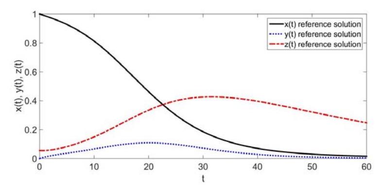
Figure 2 Reference solutions based on the ode45 algorithm in the MATLAB software, where the relative tolerance is 2.22045 ൈ 10ିଵସ and the absolute tolerance is 10ିଵହ.
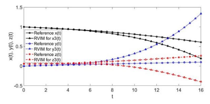
Figure 3 RVIM solutions at the third iteration. RVIM solutions are outside the normalized range ሾ0,1ሿ.
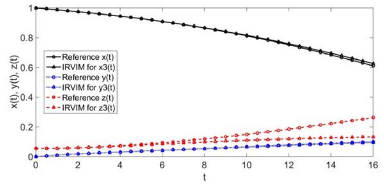
Figure 4 IRVIM's solutions at the third iteration. IRVIM's solutions are inside the normalized range ሾ0,1ሿ.
5 Conclusion
Four research goals were achieved. Firstly, we provided SAM for solving the SIR model of the spread of dengue fever in the case of South Sulawesi. Secondly, we showed that SAM is identical with RVIM. Thirdly, we proposed a modification to RVIM to obtain IRVIM. Fourthly, by computational experiments we showed that IRVIM is more accurate than RVIM. Here we note that even though both RVIM and IRVIM are quite accurate for short time periods, the solutions produced using IRVIM are more accurate and more realistic. To conclude, when we want to obtain an explicit solution to the SIR model of dengue fever disease transmission, we strongly recommend the use of the Improved Rangkuti's Variational Iteration Method (IRVIM), which was proposed in this paper.
Acknowledgement
This work was financially supported by Sanata Dharma University, which is gratefully acknowledged by the author.