
1 Introduction
The Adomian decomposition method (ADM) was introduced in 1980 to solve many linear and nonlinear equations effectively and accurately, with easy solutions of ordinary or partial differential equations with approximate values that converge speedily [1]. Several studies have been proposed to modify the regular ADM for initial value problems and boundary value problems [2-3]. An error analysis of the Adomian series of non-linear differential equations was introduced in [4] and [5] used the ADM to solve coupled systems of non-linear physical equations, coupled systems of diffusion-reaction equations and integrodifferential diffusion-reaction equations. In 2017, Nouri suggested an improvement of the ADM for the solution of stochastic differential equations [6].
Yan in 2003 proposed extended Jacobian elliptic functions to construct new exact solutions from periodic solutions of the Hirota-Satsuma coupled KdV
system by using the concept of symbolic computation [7]. Hu and Liu in 2008 proposed positon, complexiton and negaton solutions for the Hirota-Satsuma coupled KdV system, where the approximate complexiton solutions are singular and given both graphically and analytically [8]. Khater, et al. in 2017 proposed the exact traveling solution of the Hirota-Satsuma coupled KdV system depending on the modified simple equation method [9]. Hosseini, et al. in 2012 proposed an analytic method that efficiently solves ODEs, where the proposed method requires only the calculations of the first Adomian polynomial and does not need to solve the functional equations in each iteration [10]. Moradweysi, et al. in 2018 studied the pull-in instability of doubly clamped nano-switches subjected to electrostatic and intermolecular forces and proposed to solve the obtained equation by using the modified ADM [11-12].
The basic idea of the proposed FFA_MADM is to find the best parameters for the non-linear Hirota-Satsuma coupled KdV system by using the firefly algorithm (FFA), one of the most popular metaheuristic algorithms, with the modified ADM by formulating a fitness function from the modified ADM that is minimized by the FFA to attain optimal values for all parameters of the nonlinear Hirota-Satsuma coupled KdV system.
In Section 2 of this paper the mathematical model and related work are presented. In Section 3 the basic ideas of the MADM are described. In Section 4 a brief introduction of FFA is given. Section 5 is devoted to solving a nonlinear Hirota-Satsuma coupled KdV system by MADM. Section 6 describes the proposed method. Concluding remarks are given in Section 7.
2 Mathematical Model and Related Works
The coupled Korteweg-de Vries equation (CKdV) is known as [13]:
\[\frac{\partial u}{\partial t} = a \left( \frac{\partial^3 u}{\partial x^3} + 6u \frac{\partial u}{\partial x} \right) + 2bv \frac{\partial v}{\partial x},\tag{1}\]
\[\frac{\partial v}{\partial t} = -\frac{\partial^3 v}{\partial^3 x} - 3u \frac{\partial v}{\partial x} \tag{2}\] where a and b are subjective constants. The CKdV condition describes connections of two long waves with various scattering relations. It is associated in particular with most sorts of long waves with frail scattering [14-15]. By utilizing the Hirota technique, the single lone wave arrangement of this framework is:
\[u(x,t) = 2\lambda^{2} \operatorname{sech}^{2}(\varepsilon), \qquad v(x,t) = \frac{1}{2\sqrt{w}} \operatorname{sech}(\varepsilon),\]
\[\varepsilon = \lambda(x - \lambda^{2}t) + \frac{1}{2\log(w)}, \qquad w = \frac{-b}{8(4a+1)\lambda^{4}},\]
(3)
where w is an arbitrary constant depending on the parameter value \(\lambda > 0\), \(b \neq 0\) and a is any parameter such that \(4a + 1 \neq 0\).
Raslan [16] proposed the use of the ADM for a Hirota-Satsuma coupled KdV equation and a coupled MKdV equation. The local existence and smoothing properties for Hirota-Satsuma systems is discussed in [17]. Periodic solutions to generalized Hirota-Satsuma coupled systems using trigonometric and hyperbolic functions are discussed in [18]. Ismail and Ashi [19] used the Petrov-Galerkin method with a product approximation technique to numerically solve a Hirota-Satsuma coupled KdV equation.
Recently, several researchers have employed FFA to solve differential equations. Raja [20] applied ANN with other heuristic techniques to solve the one-dimensional Bratu equation. Apostolopoulos and Vlachos [21] used FFA for solving the economic emission load dispatch problem. Yang [22] has shown how to use a recently developed FFA to solve nonlinear design problems. Yang, et al. [23-24] used the firefly algorithm (FA) to determine a feasible optimal solution for the economic dispatch problem with valve loading effect problems.
3 The Modified Adomian Decomposition Method (MADM)
Suppose the general equation can be defined as follows:
\[Lu + Nu + Ru = f(x) (4)\] where L represents an invertible linear operator, N is a non-linear operator and R is the residual linear part. Then:
\[Lu = f(x) - Nu - Ru\]
If the initial conditions are used and the inverse operator \(L^{-1}\) is applied to both sides of Equation (4), we find that:
\[u = g(x) - L^{-1}Nu - L^{-1}Ru\] (5)
where \(L^{-1} = \int_0^x (.) ds\), and g(x) are the terms gotten from integrating the remaining term, f(x). The ADM expects that the nonlinear administrator N(u) can be disintegrated by an infinite series of polynomial functions given by:
\[N(u) = \sum_{n=0}^{\infty} A_n(u_0, u_1, \dots, u_n)\] where \(A_n\) are the Adomian polynomials (ADMP) [1,5]:
\[A_n = \frac{1}{n!} \frac{d^n}{d\lambda^n} \left[ N \left( \sum_{i=0}^{\infty} \lambda^i u_i \right) \right]_{\lambda=0}, \qquad n = 0, 1, 2, \dots\] (6)
El-Kalla [4] presented another formula for ADMP. He asserted that the Adomian arrangement utilizing this new approach is speedier than utilizing
ADMP Eq. (6). The Kalla polynomial in the accompanying structure is expressed as follows:
\[A_{n} = N(S_{n}) - \sum_{i=0}^{n-1} A_{i}(u_{o}, u_{1}, \dots, u_{n-1})\] where \(S_{n} = u_{o} + u_{1} + \dots + u_{n}\) and \(A_{n}\) can be given as \(A_{0} = N(u_{o})\) \[A_{1} = \frac{d}{dx} (N(u_{o}))u_{1} + \frac{1}{2} \frac{d^{2}}{dx^{2}} (N(u_{o}))u_{1}^{2} + \frac{1}{6} \frac{d^{3}}{dx^{3}} (N(u_{o}))u_{1}^{3} + \frac{1}{24} \frac{d^{4}}{dx^{4}} (N(u_{o}))u_{1}^{4} + \dots\] \[A_{2} = \frac{d}{dx} (N(u_{o}))u_{2} + \frac{1}{2} \frac{d^{2}}{dx^{2}} (N(u_{o}))[2u_{1} u_{2} + u_{2}^{2}] + \frac{1}{6} \frac{d^{3}}{dx^{3}} (N(u_{o}))[3u_{1}^{2}u_{2} + 3u_{1}u_{2}^{2} + u_{2}^{3}] + \dots\] \[(7)\]
4 Firefly Algorithm (FFA)
In recent years, researchers have been very interested in studying swarm algorithms, which have been applied for solutions to many complex applications. The firefly algorithm, developed by Yang in 2008, is one of the most important swarm algorithms and has managed to outperform many other algorithms in solving problems efficiently [25-26].
FFA has shown effectiveness and good performance in several optimization problems. The idea for FFA was inspired by the flashing light behavior of fireflies. The flashes are used as a signal system for fireflies to attract other fireflies through the characteristics of their flashing [27].
Each member of the FFA is classified as a candidate solution within the search space of the problem, while the best solutions represent the brightest locations. The attractiveness of a firefly is determined by its brightness, which is expressed in the objective function of the problem. The greater the distance between the firefly and the target location, the higher the brightness ratio [28]. At first the fireflies move randomly. During the search they are attracted to new locations (candidate solutions).
The process of attraction between the fireflies is based on the brightness of their flashes. The least bright fireflies are attracted to the brightest fireflies [29]. The mathematical representation of the FFA is determined by the size of the population in the swarm \((n_f)\), which is randomly distributed, as well as the position vector of each firefly, denoted by \(x_i = \{x_{i1}, x_{i2}, ..., x_{iD}\}\), where \(i = 1, 2, ..., n_f\), D is the dimensionality of the solutions. The distance in the search area between any two fireflies i and j at positions \(x_i\) and \(x_j\) can be calculated by the following equation:
Create objective function, positions of FFA,
Create max iteration, light intensity ,,
while (t < Max NO. of iterations).
for i=1: n (n is the No. of fireflies)
for j=1: n (n is the No. of fireflies)\nif move firefly towards\nendif
Evaluate the new solutions in FFA
Update the light intensity equation.\nend for j\nend for i
Update the current best solution\nend while
Return the current best solution results
End
Figure 1 Pseudocode of the FFA.
\[r_{ij} = ||x_i - x_j|| = \sqrt{\sum_{D=1}^{Dim} (x_{iD} - x_{jD})^2}, i \neq j, \text{ and } i, j = 1, 2, ... n\] (8)
where Dim represents the dimensions of the solutions to the problem.
The value of the objective function represents the brightness of firefly i at position \(x_i\), which is calculated by the following equation:
\[I_f(x_i) = F(x_i) \tag{9}\]
The intensity depends on the \(I_{f0}\) emitted and the distance \(r_{ij}\) between the fireflies. The light intensity \(I_f(r)\) can be described by \(r_{ij}\) as follows [27]:
\[I_f(r) = I_{f0}e^{-\gamma^{rm}}, \qquad m \ge 1\] (10)
where \(\gamma\) can be taken as a constant.
Each firefly has a certain attractiveness in the swarm and \(\beta_f\) varies relative to distance \(r_{ij}\). The main formula for the attractiveness of a firefly is formulated as follows [30]:
\[\beta_f(r) = \beta_{f0} e^{-\gamma^{r^m}}, \qquad m \ge 1 \tag{11}\] where \(\beta_f(r)\) is the attractiveness function at distance r and \(\beta_{f0}\) is the initial attractiveness of the firefly (which can be constant). Firefly positions are updated in the swarm depending on their brightness. A less bright firefly \(x_i\)
moves towards a brighter firefly \(x_j\) because of attraction. The equation of movement is defined as follows:
\[x_{id}^{t+1} = x_{id}^{t} + \beta_{f0} e^{-\gamma^{r^{m}}} (x_{id}^{t} - x_{id}^{t}) + \alpha_{t} \varepsilon_{id}^{t}\] (12)
where \(\alpha_t\) is a random parameter, \(\gamma\) is the coefficient, and id = (rand - 0.5), where 'rand' represents a random number from an uniform distribution in the interval [0,1]. The pseudocode for the FFA can be written as in Figure 1 [31].
5 Application of MADM to the Coupled Hirota-Satsuma System
This section is devoted to the analytical solution of Hirota-Satsuma Eq. (1) and Eq. (2). For this purpose, MADM was used in order to obtain the solution.
Let the standard form of Equations Eq. (1-2) in an operator be:
\[L_t u - a L_{xxx} u - 6au L_x u - 2b v L_x v = 0, (13)\]
\[L_t v + L_{rrr} v + 3 u L_r v = 0, (14)\]
\[u(x,0) = g_1(x)\]
\[v(x,0) = g_2(x)\] where the notations \(L_t = \frac{\partial}{\partial t}\), \(L_x = \frac{\partial}{\partial x}\) and \(L_{xxx} = \frac{\partial^3}{\partial x^3}\) symbolize the linear differential operator.
Let \(L_t^{-1}\) be the inverse of operator \(L_t\). It can conveniently be taken as an integral with respect to t from 0 to t.
Define \(L_t^{-1} = \int_0^t (.) dt\). Then system Eqs. (8-9) becomes:
\[u(x,t) = g_1(x) + L_t^{-1} [a L_{xxx} u + 6a \emptyset_1(u) + 2b \emptyset_2(v)],\] (15)
\[v(x,t) = g_2(x) - L_t^{-1}[L_{xxx}v + 3\emptyset_3(u,v)],\] (16)
where:
\[\emptyset_1(u) = u u_r, \qquad \emptyset_2(v) = v v_r, \qquad \emptyset_3(u,v) = u v_r\]
MADM assumes an infinite series for the unknown functions u(x,t) and v(x,t) in the form
\[u(x,t) = \sum_{n=0}^{\infty} u_n(x,t), \qquad v(x,t) = \sum_{n=0}^{\infty} v_n(x,t),\] (17)
We can write \(\emptyset_1\), \(\emptyset_2\), and \(\emptyset_3\) by an infinite series of Adomian polynomials in the form
\[\emptyset_1(u) = \sum_{n=0}^{\infty} A_n, \quad \emptyset_2(v) = \sum_{n=0}^{\infty} B_n, \quad \emptyset_3(u, v) = \sum_{n=0}^{\infty} C_n\] (18)
where \(A_n\), \(B_n\), and \(C_n\) are the appropriate ADMP. That is, when \(A_n\), \(B_n\), and \(C_n\) are the appropriate Adomian polynomials, the general form of the formulas is:
\[A_n(u_0, u_1, ..., u_n) = \frac{1}{n!} \frac{d^n}{dv^n} \left[ \emptyset_1 \left( \sum_{k=0}^{\infty} \gamma^k u_k \right) \right]_{\gamma=0}, n \ge 0\] (19)
\[B_n(v_o, v_1, ..., v_n) = \frac{1}{n!} \frac{d^n}{dv^n} \left[ \emptyset_2 \left( \sum_{k=0}^{\infty} \gamma^k v_k \right) \right]_{\gamma=0} , n \ge 0\] (20)
\[C_{n}(u_{o}, u_{1}, ..., u_{n}, v_{o}, v_{1}, ..., v_{n}) = \frac{1}{n!} \frac{d^{n}}{d\gamma^{n}} \left[ \emptyset_{3} \left( \sum_{k=o}^{\infty} \gamma^{k} u_{k}, \sum_{k=o}^{\infty} \gamma^{k} v_{k} \right) \right]_{\gamma=0},\] \[n \geq 0\] (21)
For example, the first polynomials using Eq. (14) and Eq. (16) are computed as follows:
\[A_{0} = u_{0} \frac{\partial u_{0}}{\partial x}\] \[A_{1} = u_{0} \frac{\partial u_{1}}{\partial x} + u_{1} \frac{\partial u_{0}}{\partial x} + u_{1} \frac{\partial u_{1}}{\partial x}\] \[A_{2} = u_{0} \frac{\partial u_{2}}{\partial x} + u_{2} \frac{\partial u_{0}}{\partial x} + u_{2} \frac{\partial u_{1}}{\partial x} + u_{1} \frac{\partial u_{2}}{\partial x} + u_{2} \frac{\partial u_{2}}{\partial x}\] \[A_{3} = u_{3} \frac{\partial u_{0}}{\partial x} + u_{0} \frac{\partial u_{3}}{\partial x} + u_{3} \frac{\partial u_{1}}{\partial x} + u_{1} \frac{\partial u_{3}}{\partial x} + \cdots\] \[A_{4} = u_{4} \frac{\partial u_{0}}{\partial x} + u_{0} \frac{\partial u_{4}}{\partial x} + \cdots\] \[\vdots\] \[B_{0} = v_{0} \frac{\partial v_{0}}{\partial x}\] \[B_{1} = v_{0} \frac{\partial v_{1}}{\partial x} + v_{1} \frac{\partial v_{0}}{\partial x} + v_{1} \frac{\partial v_{1}}{\partial x}\] \[B_{2} = v_{0} \frac{\partial v_{2}}{\partial x} + v_{2} \frac{\partial v_{0}}{\partial x} + v_{2} \frac{\partial v_{1}}{\partial x} + v_{1} \frac{\partial v_{2}}{\partial x} + v_{2} \frac{\partial v_{2}}{\partial x}\] \[B_{3} = v_{3} \frac{\partial v_{0}}{\partial x} + v_{0} \frac{\partial v_{3}}{\partial x} + v_{3} \frac{\partial v_{1}}{\partial x} + v_{1} \frac{\partial v_{3}}{\partial x} + \cdots\] \[\vdots\] \[C_{0} = u_{0} \frac{\partial v_{0}}{\partial x}\] \[C_{1} = u_{0} \frac{\partial v_{0}}{\partial x} + u_{1} \frac{\partial v_{0}}{\partial x} + u_{1} \frac{\partial v_{1}}{\partial x}\] \[C_{2} = u_{0} \frac{\partial v_{2}}{\partial x} + u_{2} \frac{\partial v_{0}}{\partial x} + u_{2} \frac{\partial v_{1}}{\partial x} + u_{1} \frac{\partial v_{2}}{\partial x} + u_{2} \frac{\partial v_{2}}{\partial x}\] \[C_{3} = u_{3} \frac{\partial v_{0}}{\partial x} + u_{0} \frac{\partial v_{3}}{\partial x} + u_{3} \frac{\partial v_{1}}{\partial x} + u_{1} \frac{\partial v_{3}}{\partial x} + \cdots\] and so on. The nonlinear systems Eqs. (15-16) are constructed as follows:
\[u_{o}(x,t) = g_{1}(x), v_{o}(x,t) = g_{2}(x),\] \[u_{n+1}(x,t) = L_{t}^{-1}[a L_{xxx}u_{n} + 6a A_{n} + 2b B_{n}]; n \ge 1 (22)\] \[v_{n+1}(x,t) = -L_{t}^{-1}[L_{xxx}v_{n} + 3 C_{n}]; n \ge 1 (23)\] where the functions \(g_1(x)\) and \(g_2(x)\) are the initial condition. We construct the solution u(x,t) and v(x,t) as follows:
\[\lim_{n\to\infty}\psi_n=u(x,t),\qquad \lim_{n\to\infty}\varphi_n=v(x,t)\] where:
\[\psi_n(x,t) = \sum_{k=0}^n u_k(x,t), \qquad \varphi_n(x,t) = \sum_{k=0}^n v_k(x,t),\] (24)
and the recurrence relation is given as in Eqs. (22-23).
To examine the performance of MADM for solving Eqs. (1-2), we set the initial condition [16]:
\[u_o(x,t) = 2\lambda^2 \operatorname{sech}^2\left(\lambda x + \frac{1}{2ln(w)}\right), \quad v_o(x,t) = \frac{1}{2} \frac{\left(\lambda x + \frac{1}{2ln(w)}\right)}{\sqrt{w}}\] where w is an arbitrary constant depending on parameter value \(\lambda > 0\), \(b \neq 0\) and a is any parameter such that \(4a + 1 \neq 0\). Now, the reclusive relation can be written as follows:
\[\text{[rumus tidak dapat ditampilkan dengan baik — lihat PDF asli]}\]
\[\cosh\left(\frac{1}{2} \frac{2\lambda \ln(w) x + 1}{\ln(w)}\right)^{3} wab + 18 \lambda^{2} t^{3} \sinh\left(\frac{1}{2} \frac{2\lambda \ln(w) x + 1}{\ln(w)}\right) ab^{2}\] (25) \[v(x,t) = v_{0}(x,t) + v_{1}(x,t) + v_{2}(x,t) \dots = \frac{1}{8} \frac{1}{w^{\frac{3}{2}} \cosh\left(\frac{1}{2} \frac{2\lambda \ln(w) x + 1}{\ln(w)}\right)^{6}} \left(4 \cosh\left(\frac{1}{2} \frac{1}{\ln(w)} (2\lambda \ln(w) x + 1)\right)^{5}\right) w + 4\lambda^{3} \sinh\left(\frac{1}{2} \frac{2\lambda \ln(w) x + 1}{\ln(w)}\right) t\left(\frac{1}{2} \frac{1}{(\ln(w)) (2\lambda \ln(w) x + 1)}\right)^{4} - 64 \lambda^{9} t^{3} \sinh\left(\frac{1}{2} \frac{2\lambda \ln(w) x + 1}{\ln(w)}\right) aw \cosh\left(\frac{1}{2} \frac{1}{(\ln(w))} (2\lambda \ln(w) x + 1)\right)^{2}\] (26)
6 Firefly Proposed Method (FFA MADM)
The idea of the proposed FFA_MADM method is based on finding the best and optimal parameters for nonlinear Hirota-Satsuma systems using FFA combined with MADM. The results of MADM solution series Eqs. (25-26) are used to formulate the objective or fitness function in the FFA using:
\[U(a,b,\lambda) = MSE\left(\sum_{i=1}^{n} \sum_{j=1}^{m} \left(u(x_i,t_j) - \hat{u}(x_i,t_j)\right)^2\right)\](27)
\[V(a,b,\lambda) = MSE\left(\sum_{i=1}^{n} \sum_{j=1}^{m} \left(v(x_i,t_j) - \hat{v}(x_i,t_j)\right)^2\right)\](28)
\[F = \min \frac{1}{2} |U(a, b, \lambda) + V(a, b, \lambda)| \tag{29}\] where F represents the fitness function (MSE) solved by using FFA, n and m represent the total number of steps used in the solution domain of x and t respectively, u and v are the solutions of nonlinear Hirota-Satsuma systems Eqs. (25-26), \(\hat{u}\) and \(\hat{v}\) are the exact solutions for these systems. Consequently, the best values for systems Eqs. (25-26) are obtained from the following parameter values:
\[a = -2.7286.\]
\(b = 4.4061.\)
\(\lambda = -0.0086.\)
The proposed method supposes an elementary standard model structure where some of the parameters are unknown. The objective of this method is to find the optimal parameters \((a, b, \lambda)\) for nonlinear Hirota-Satsuma coupled KdV systems to minimize the differences between the model output vector and the real response vector.
The default settings for the FFA parameters listed in Table 1 were used by the Matlab® R2016a software.
Table 1 Parameter Values for FFA
| Parameter Name | Values | |
|---|---|---|
| Swarm size | 30 | |
| Max no. of iterations | 500 | |
| Max stall generations | 50 | |
| Initial population range | [-10, 10] | |
| Number of decision variables | 3 | |
| Light absorptioncCoefficient | 1 | |
| Attraction coefficient | 2 | |
| Mutation coefficient | 0.2 | |
We note that the proposed FFA_MADM algorithm outperformed the numerical method both at t=0.5 and t=1 as can be seen in comparison of absolute errors using 2, see Table 2.
Table 2 Comparison of Absolute Errors Using 2 for Various Values of and in Hirota-Satsuma System between FFA_MADM and MADM
| FFA_MADM | MADM | FFA_MADM | MADM | |
|---|---|---|---|---|
| x | t = 0.5 | t = 1 | ||
| 0 | 8.2799e-24 | 8.1547e-6 | 4.3946e-23 | 3.3335e-5 |
| 0.1 | 7.9989e-24 | 1.3822e-5 | 4.2685e-23 | 8.4115e-5 |
| 0.2 | 7.7207e-24 | 2.0346e-5 | 4.1426e-23 | 1.4248e-4 |
| 0.3 | 7.4454e-24 | 2.7423e-5 | 4.0170e-23 | 2.0566e-4 |
| 0.4 | 7.1730e-24 | 3.4660e-5 | 3.8915e-23 | 2.7011e-4 |
| 0.5 | 6.9035e-24 | 4.1623e-5 | 3.7662e-23 | 3.3203e-4 |
| 0.6 | 6.6368e-24 | 4.7890e-5 | 3.6412e-23 | 3.8778e-4 |
| 0.7 | 6.3730e-24 | 5.3102e-5 | 3.5163e-23 | 4.3428e-4 |
| 0.8 | 6.1122e-24 | 5.6994e-5 | 3.3917e-23 | 4.6928e-4 |
| 0.9 | 5.8542e-24 | 5.9407e-5 | 3.2673e-23 | 4.9149e-4 |
| 1 | 5.5991e-24 | 6.0302e-5 | 3.1431e-23 | 5.0058e-4 |
| MSE | 4.8576e-47 | 1.8077e-9 | 1.4348e-45 | 1.1866e-7 |
Figure 2 depicts the absolute error of the Hirota-Satsuma system by U equation at t=0.5 and t=1.
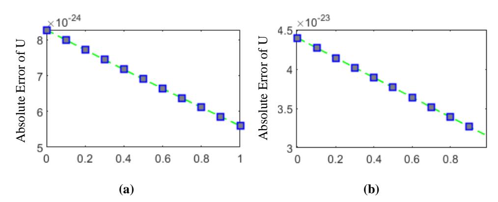
Figure 2 Absolute error of the Hirota-Satsuma system by: (a) U equation when t = 0.5, (b) U equation when t = 1.
The proposed FFA_MADM algorithm also outperformed the numerical method at both t=0.5 and t=1 as shown in comparison of absolute errors using v2, see Table 3.
Table 3 Comparison of Absolute Errors Using 2 for Various Values of and in Hirota-Satsuma System between FFA_MADM and MADM
| FFA_MADM | MADM | FFA_MADM | MADM | |
|---|---|---|---|---|
| x | t = 0.5 | t = 1 | ||
| 0 | 2.1884e-24 | 1.9191e-5 | 5.6782e-24 | 1.5662e-4 |
| 0.1 | 2.0998e-24 | 2.1578e-5 | 5.4934e-24 | 1.7534e-4 |
| 0.2 | 2.0127e-24 | 2.2771e-5 | 5.3101e-24 | 10844e-4 |
| 0.3 | 1.9273e-24 | 2.2785e-5 | 5.1284e-24 | 1.8411e-4 |
| 0.4 | 1.8434e-24 | 2.1718e-5 | 4.9482e-24 | 1.7508e-4 |
| 0.5 | 1.7611e-24 | 1.9730e-5 | 4.7695e-24 | 1.5870e-4 |
| 0.6 | 1.6804e-24 | 1.7026e-5 | 4.5923e-24 | 1.3660e-4 |
| 0.7 | 1.6012e-24 | 1.3831e-5 | 4.4167e-24 | 1.1061e-4 |
| 0.8 | 1.5237e-24 | 1.0369e-5 | 4.2426e-24 | 8.2539e-5 |
| 0.9 | 1.4478e-24 | 6.8489e-6 | 4.0701e-24 | 5.4042e-5 |
| 1 | 1.3734e-24 | 3.4455e-6 | 3.8991e-24 | 2.6544e-5 |
| MSE | 3.1958e-48 | 3.0727e-10 | 2.3137e-47 | 2.0034e-8 |
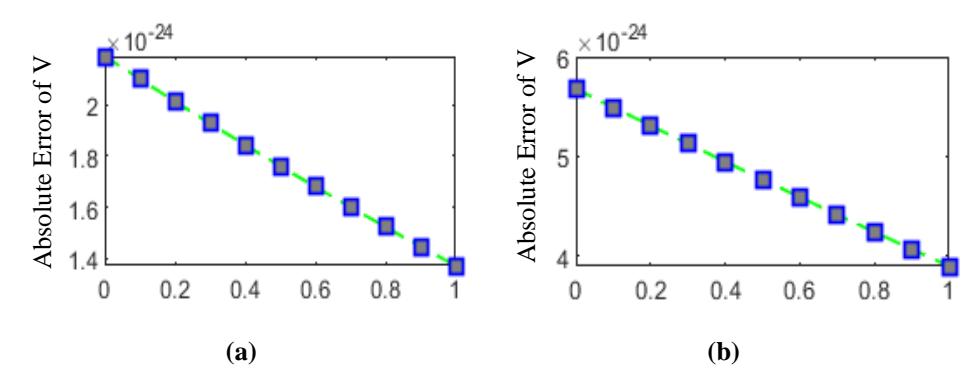
Figure 3 The absolute error of the Hirota-Satsuma system by: (a) V equation when t = 1, (b) V equation when t = 1.
7 Conclusion
In this paper, nonlinear Hirota-Satsuma coupled KdV systems were solved using MADM combined with FFA. The basic idea for the proposed hybrid method is to find the optimal parameters for nonlinear Hirota-Satsuma coupled KdV systems \((a,b,\lambda)\) as they are widely applied to solve other nonlinear systems. Compared to MADM, FFA_MADM ensures that the optimal parameters will be appropriately selected even if the system has multiple values and gives more accurate results than MADM. The tables and figures in this paper indicate that the approximate solutions obtained by FFA_MADM were in great agreement with the exact solutions. The calculations in this paper were performed using the MAPLE 13 and the Matlab® R2016a software.
Acknowledgments
This work was supported by the Mosul University, College of Computer Sciences and Mathematics, Republic of Iraq.