
1 Introduction
The World Health Organization states that infectious diseases may be caused by bacteria, viruses or other pathogens [1]. An increase in the population of such organisms may increase the number of infectious disease cases. Also, the number infections is correlated with the number of contacts. Epidemic models can be used to analyze the spread of infectious diseases. The models themselves are often expressed in terms of differential equation systems that describe the growth rate of the state variables within the system.
In 1927, Kermack and Mckendrick presented the SIR epidemic model. This model describes the phenomenon of a disease spreading among susceptible individuals who become infected when they have contact with infected
individuals and who may recover following treatment [2]. In 2017, Cai et al. introduced a modification of the SIR model, namely the SIRS epidemic model, which uses a nonlinear incidence rate [3]. This model showed that recovered individuals may become susceptible again.
One disease that allows recovered individuals to become susceptible again is tuberculosis. Tuberculosis is an infectious disease caused by the bacteria Mycobacterium tuberculosis [4]. The WHO has states that tuberculosis is one of the top 10 causes of death in the world [5]. The tuberculosis bacteria can remain dormant for years and become active again; the incidence of secondary tuberculosis is around 90% [6]. Tuberculosis sufferers who have recovered can be infected again when there is a decrease in their immune system. Tuberculosis spreads quickly among people who have a weak immune system [7].
Epidemic models can be categorized into deterministic and stochastic models. Deterministic models are not sufficient to represent epidemic conditions in the field, so a stochastic model which considers the random effects of uncertain cases is needed [8]. The stochastical model developed by Cao et al. [9] in 2019 (SIQR) showed what happens when there is a quarantining process for infected individuals.
The SIQR model uses the Stochastic Differential Equation (SDE) to know the influence of white noise in a stochastic system. They verified if there is a stationary distribution under certain conditions. The SIQR model of Cao et al. does not describe a specific kind of infectious disease and they did not discuss the transition and outbreak probabilities in their paper. In essence, the state of the number of individuals is a discrete random variable when time is continuous. The present research examined a model of disease spread with a different approach, namely using the CTMC (Continuous Time Markov Chain). The SIQR model of Cao et al. was modified to become the SIQRS model, which was applied to tuberculosis. The purposes of this study were: (1) to modify the SIQR model into the SIQRS model; (2) to determine the transition probability, the outbreak probability and the expected time until disease extinction using the CTMC approach; and (3) to simulate the effect of quarantining on the expected time until disease extinction.
2 Mathematical Model
The mathematical model used in this article is a modification of the SIQR model into the SIQRS model. The modification of the SIQR model into SIQRS was carried out because sufferers of some diseases can become susceptible again after having recovered. The SIQRS model consists of four subpopulations, i.e. susceptible individuals (), infected individuals (), quarantined individuals (Q), and recovered individuals (R). The total of population is assumed constant. Then, N(t) = N and the birth rate is the same as the death rate. A compartment diagram of the model is shown in Figure 1.
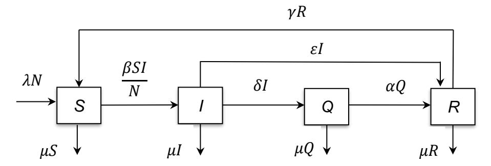
Figure 1 Compartment diagram of the deterministic SIQRS model, which is a modification of the SIQR model, which considers that recovered individuals may become susceptible again.
Based on the compartment diagram in Figure 1, the ordinary differential equation system of the SIQRS model was obtained:
\[\frac{dS(t)}{dt} = \lambda N - \mu S(t) - \frac{\beta S(t)I(t)}{N(t)} + \gamma R(t)\] \[\frac{dI(t)}{dt} = \frac{\beta S(t)I(t)}{N(t)} - (\varepsilon + \mu + \delta)I(t)\] \[\frac{dQ(t)}{dt} = \delta I(t) - (\mu + \alpha)Q(t)\] \[\frac{dR(t)}{dt} = \varepsilon I(t) + \alpha Q(t) - (\mu + \gamma)R(t)\] (1)
The parameters \(\lambda\), \(\mu\), \(\beta\), \(\varepsilon\), \(\delta\), \(\alpha\), \(\gamma\) are positive values and N = S(t) + I(t) + Q(t) + R(t) for all \(t \ge 0\). A description of each parameter is presented in Table 1.
| Parameters | Description | |
|---|---|---|
| λ | Birth rate | |
| \(\mu\) | Death rate | |
| β | Transmission rate | |
| \(\varepsilon\) | Rate of healing without quarantine treatment | |
| δ | Quarantine rate | |
| \(\alpha\) | Rate of healing with quarantine treatment | |
| γ | Rate of entry of recovered individuals back into the susceptible class | |
| N | Total population number | |
Table 1 List of parameters in the SIQRS model.
3 CTMC Stochastic SIQRS Model
3.1 Transition Probability
The transition probability is the probability of a stochastics process moving from state to state . Here, the stochastic SIQRS model consists of three random variables, i.e. (),(),(). () is the size of the total population, which is assumed to be constant. Then () = for all ≥ 0 where () = () + () + () + (). Thus, variable () is determined by () = () − () − () − (), where is time. Suppose an ordered pair ((),(),())=(, , ) and (( + ∆),( + ∆),( + ∆) = (, , ) where , , , , , = 0,1,2 …. Then based on Allen [8] the transition probability for the SIQRS model can be formulated as follows:
\[Prob_{(k,l,m),(s,i,q)}(t,t+\Delta t) = Prob\{S(t+\Delta t) = k, I(t+\Delta t) = l, Q(t+\Delta t) = m | (S(t) = s, I(t) = i, Q(t) = q)\}\] \[\begin{cases} (\lambda N + \gamma R)\Delta t + o(\Delta t), (k, l, m) = (s+1, i, q) \\ \left(\frac{\beta SI}{N}\right)\Delta t + o(\Delta t), (k, l, m) = (s-1, i+1, q) \\ (\mu S)\Delta t + o(\Delta t), (k, l, m) = (s-1, i, q) \\ (\delta I)\Delta t + o(\Delta t), (k, l, m) = (s, i-1, q+1) \\ ((\mu+\varepsilon)I)\Delta t + o(\Delta t), (k, l, m) = (s, i-1, q) \\ ((\mu+\alpha)Q)\Delta t + o(\Delta t), (k, l, m) = (s, i, q-1) \\ (1-\xi)\Delta t + o(\Delta t), (k, l, m) = (s, i, q) \\ o(\Delta t), \text{ otherwise} \end{cases}\] (2)
where = + + + + + ( + ) + ( + ). The transition probabilities of susceptible, infected, and quarantined individuals in the time interval ( + ∆) only depend on time , where ≥ 0. The time value ∆ is assumed to be very small so that the change occurring in susceptible, infected, and quarantined individuals is the maximum of one individual in such a short time interval ∆. The value of (∆) represents a small probability value and satisfies (∆) ∆ = 0 [8].
3.2 Outbreak Probability
Outbreak events occur when the number of infected individuals increases over time. The basic reproduction number (0) and the expected number of infected individuals () are used as criteria for the occurrence of disease outbreaks in the long term. The basic reproduction number (0) is the number of susceptible individuals getting infected after an infected individual is introduced into the system. Based on Basir et al. [10], the value of 0 for the SIQRS model is 0 = (++) . The basic reproduction number (0) has the same definition as the expected number of infected individuals (), which is calculated using a probability method. In deterministic models, disease outbreak events occur when 0 > 1, whereas in stochastic models this is associated with a condition when the expected number of infected individuals () > 1. Basic reproduction number (0) and are obtained with different approaches. If 0 > 1 it cannot be ascertained if > 1, both are just similar. The outbreak probability and the expected number of infected individuals is obtained through a branching process approach [8]. The benchmark for the outbreak probability is determined by the expected number of infected individuals (), not from the basic reproduction number (0). Based on this process, the SIQRS model has the following disease extinction probabilities:
\[Prob\{I(t) = 0\} = \begin{cases} 1 \ ; m \le 1 \\ \tau \ ; m > 1, \end{cases}\] (3)
Consequently, the probability of an outbreak occurring is:
\[1 - Prob\{I(t) = 0\} = \begin{cases} 0 & ; m \le 1\\ 1 - \tau ; m > 1, \end{cases}\] (4)
where
\[\tau = \left(\frac{N}{sR_0}\right)^{i_0}.\tag{5}\]
3.3 Expected Time Until Disease Extinction
The expected time until disease extinction is the time it takes for the disease to disappear. Based on Syams [11], the expected time until disease extinction can be determined by generator matrix . Generator matrix gives the rate of transition [8], which can be derived from the transition probability. Suppose the transition probabilities () = (()) are assumed to be continuous, differentiable for ≥ 0. Then, at = 0, (0) = 0, ≠ and (0) = 1. The derivation of the transition probability can be expressed as:
\[\frac{dp}{dt} = Qp,\tag{6}\] where = () is the rate of transition from state to state and can be expressed as:
\[Q = \begin{pmatrix} q_{00} & q_{01} & q_{02} & \cdots \\ q_{10} & q_{11} & q_{12} & \cdots \\ q_{20} & q_{21} & q_{22} & \cdots \\ \vdots & \vdots & \vdots & \vdots \end{pmatrix}\] (7)
The formula to determine the expected time until disease extinction by generator matrix Q is as follows:
\[\tau = cO^{-1},\tag{8}\] where c = (0, -1, -1, ..., -1), and \(Q^{-1}\) is the inverse of generator matrix Q. If the population is small, such as 3, 4, or 5 people, it can be obtained by that formula, but if the population number is large, then generator matrix Q is difficult to obtain [11].
In this study, because the population number that was simulated was large, a computer simulation was carried out with 100 trials to get the expected time until disease extinction. The number of 100 trials was selected because it is sufficient to get the probability distribution of the expected time of disease extinction from a manual simulation. The 100 trials were performed for different quarantine rates \((\delta)\), i.e. \(\delta=0.1\), \(\delta=0.2\), \(\delta=0.4\), \(\delta=0.6\), \(\delta=0.8\), and \(\delta=1\) to get the distribution of the disease extinction probability for each parameter value. Thus, the expected time until disease extinction could be obtained from this distribution by multiplying the middle point of the time interval with its probability.
4 Numerical Simulation
Numerical simulations were carried out to describe the spread of an infectious disease, namely tuberculosis, by applying the SIQRS model. In particular, simulations were carried out to determine the effect of quarantine on the expected time until disease extinction. The scenarios investigated were: (1) the effect of decreasing the healing rate (meaning the healing time increases) without quarantine; (2) the effect of increasing the transmission rate without quarantine; (3) the effect of increasing the quarantine rate on the expected time until disease extinction. In other words, the simulation was carried out by varying the values of the following parameters: healing rate without quarantine \((\varepsilon)\), transmission rate \((\beta)\), quarantine rate \((\delta)\), while the other parameter values were unchanged, i.e. birth rate \((\lambda)\), death rate \((\mu)\), rate of healing with quarantine \((\alpha)\), rate of entry of recovered individuals back into the susceptible class \((\gamma)\). This stochastic model simulation was carried out using the software package R-3.6.1 by adaptivetau. As mentioned, the parameter values used in the simulation were based on the case of tuberculosis, as presented in Table 2.
| Variable | Parameter Values | Unit | Source |
|---|---|---|---|
| μ | 0.014 | 1/year | (BPS 2020) [12] |
| λ | 0.014 | 1/year | Assumed |
| β | 0.002 | 1/year | (Kemenkes RI 2019) [13] |
| \(\varepsilon\) | (365/210) | 1/year | Assumed |
| δ | 0.5 | 1/year | Assumed |
| \(\alpha\) | (365/180) | 1/year | (Naomi et al. 2016) [14] |
| γ | (1/5) | 1/year | Assumed |
| N | 100 | person | Assumed |
Table 2 Parameter values.
The total population simulated was 100 people (N = 100) with the following initial values for susceptible, infected, quarantined, recovered individuals: S(0) = 70, I(0) = 10, Q(0) = 10, R(0) = 10, assuming that 50% of the total population was quarantined. The simulation result is shown in Figure 2.
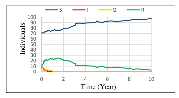
Figure 2 Population dynamics for tuberculosis.
Based on the simulation results, when the number of infected individuals and quarantined individuals was initially 10 people, after some time it will go to 0. When there are 70 susceptible individuals initially, after a while this number will continue to increase. Tuberculosis disappeared around 6-7 months, to be precise at 0.671156 years. This means that tuberculosis will not occur as an epidemic if the infected individuals are taking regular medication for 6 to 7 months and 50% of infected individuals quarantined themselves. This is consistent with analytical calculations, namely a basic reproduction number \((R_0)\) of 0.000888 < 1, which means there is no outbreak in the long term with a probability of 1. The results of this simulation were the basis for knowing the effects of changes in the values of the healing rate, the transmission rate, and the rate of quarantine influencing population dynamics.
4.1 Scenario 1: Effect of Decreasing Healing Rate Without Quarantine
Based on the initial values, it was found that the recovery time was around 6 to 7 months. With Scenario 1 it was studied what happens when the healing time is longer, that is about 1 year with = (365/365), 2 years with = (365/730), 3 years with = (365/1095), and the quarantine rate is 0, while the other parameter values were the same as those presented in Table 2. The results of analytic calculations for the basic reproduction number (0), the expected number of infected individuals () and the outbreak probability are presented in Table 3.
Table 3 Influence of on basic reproduction number, expected number of infected individuals, and outbreak probability.
| Parameter values of 𝜀 | Basic reproduction number | Expected number of infected individuals | Outbreak probability |
|---|---|---|---|
| (365/365) | 0.001972 | 0.002758 | 0 |
| (365/730) | 0.003891 | 0.005433 | 0 |
| (365/1095) | 0.005758 | 0.008029 | 0 |
Below are the simulation results for the influence of parameter :
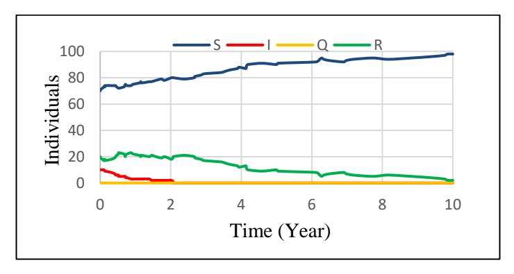
Figure 3 Dynamics of susceptible, infected, quarantined, and recovered individuals at time for = (365/365).
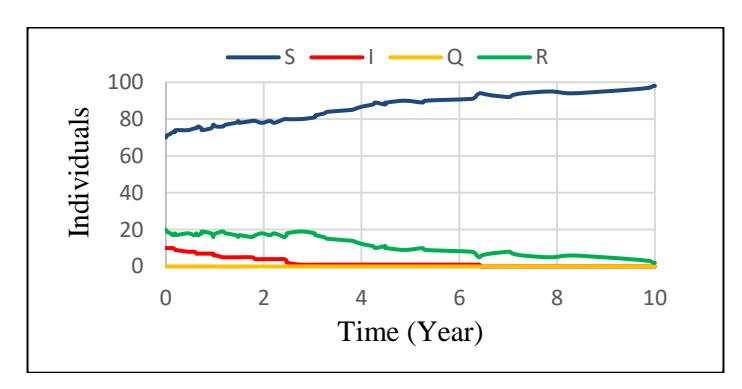
Figure 4 Dynamics of susceptible, infected, quarantined, and recovered individuals at time t for \(\varepsilon = (365/730)\).
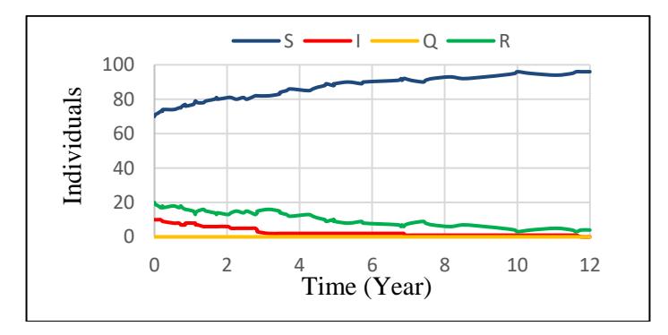
Figure 5 Dynamics of susceptible, infected, quarantined, and recovered individuals at time t for \(\varepsilon = (365/1095)\).
The simulation results in Figures 3, 4 and 5 describe that when the healing rate was decreased or the length of the healing time was increased, the number of susceptible individuals in Figures 3, 4, and 5 increased, while the number of infected and recovered individuals decreased. In Figures 3, 4, and 5 it can be seen that when the healing rate was decreased, the decrease in the number of infected individuals was slower. The time of disease extinction for tuberculosis in Figures 3, 4 and 5 was 2.07, 6.45, and 11.76, respectively. This indicates that tuberculosis will disappear slower from the population if the healing rate \((\varepsilon)\) is decreased.
Based on Table 3 it can be seen that a decrease in the healing rate increases the basic reproduction number \((R_0)\) and the expected number of infected individuals (m) even though values of \(R_0 < 1\) and m < 1 are obtained. This indicates that in the long term there will be no outbreak event, i.e. the probability of an outbreak is 0 because the number of infected individuals will
go to 0 in the same time. Based on the results of the simulation, it can be concluded that a decrease in the healing rate without quarantine will result in longer time until disease extinction.
4.2 Scenario 2: Effect of Increasing Transmission Rate Without Quarantine
In Scenario 2, based on the initial values, the simulation of the transmission rate is 0.002. With this scenario it is studied what happens when the transmission rate increases 100 times, 200 times, and 300 times. The transmission rate becomes = 0.2, = 0.4, = 0.6 and the quarantine rate is 0, while the other parameter values are the same as shown in Table 2. The basic reproduction number (0) and the expected number of infected individuals () can be used to determine whether or not an outbreak will occur in the future. The results of calculating the basic reproduction number (0), the expected number of infected individuals (), and the outbreak probability are presented in Table 4.
Table 4 Influence of on basic reproduction number, expected number of infected individuals, and outbreak probability
| Parameter values of 𝛽 | Basic reproduction number | Expected number of infected individuals | Outbreak probability |
|---|---|---|---|
| 0.2 | 0.575816 | 0.574555 | 0 |
| 0.4 | 1.151631 | 0.892667 | 0 |
| 0.6 | 1.727447 | 1.0947 | 0.850386 |
Below are the simulation results for the influence of :
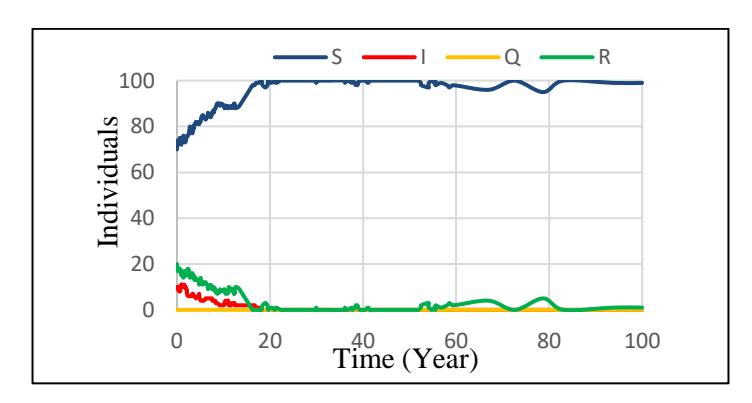
Figure 6 Dynamics of susceptible, infected, quarantined, and recovered individuals at time for = 0.2.
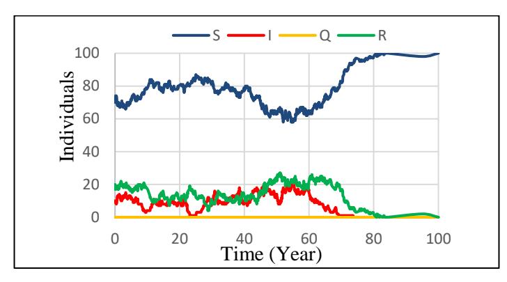
Figure 7 Dynamics of susceptible, infected, quarantined, and recovered individuals at time t for \(\beta = 0.4\).
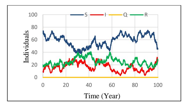
Figure 8 Dynamics of susceptible, infected, quarantined, and recovered individuals at time t for \(\beta = 0.6\).
The simulation results in Figures 6, 7 and 8 show that if \(\beta = 0.2\), the number of infected individuals decreased, with time until disease extinction time at 18.18 years. When the contact rate was increased to \(\beta = 0.4\) and \(\beta = 0.6\), the number of infected individuals fluctuated and made the disease disappear slower than in the previous simulation. Likewise, the result of the analytical calculations in Table 4 shows that an increase in the transmission rate causes an increase in the basic reproduction number \((R_0) > 1\) and the expected number of infected individuals (m) > 1, which increases the outbreak probability. Based on the result of the simulations conducted it can be concluded that an increase in the transmission rate without quarantine makes the disease disappear from the population over a longer time and allows an outbreak in the long term.
4.3 Scenario 3: Effect of Increasing the Quarantine Rate on the Expected Time until Disease Extinction
Scenario 3 was used to determine the effect of the quarantine rate on the expected time until disease extinction. At baseline, 50% of infected individuals are quarantined. In this scenario it was studied what happens when the quarantine rate was (a) = 0.1, (b) = 0.2, (c) = 0.4, (d) = 0.6, (e) = 0.8, (f) = 1. The parameter values in this simulation were the same as in Table 2 except for the values of the transmission rate (), which was 0.6, and the healing rate (), which was (365/1095). The reason for choosing these parameter values was because, based on the previous simulations, these values indicate the highest time until disease extinction compared to the previous parameter values. Below is the distribution of the probability of disease extinction from 100 trials for each value of the quarantine rate (). Based on this the expected time until disease extinction was calculated.
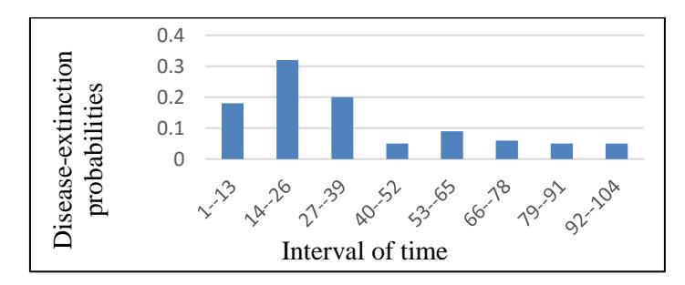
Figure 9 Disease extinction probabilities diagram for = 0.1.
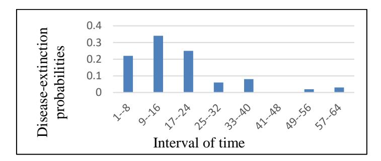
Figure 10 Disease extinction probabilities diagram for = 0.2.
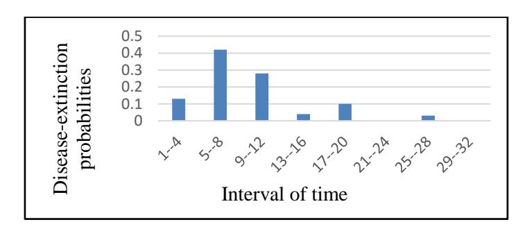
Figure 11 Disease extinction probabilities diagram for = 0.4.
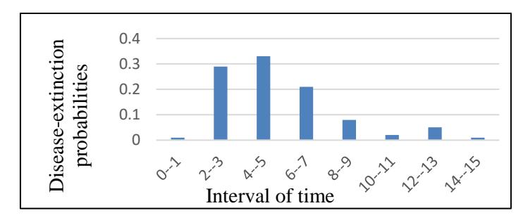
Figure 12 Disease extinction probabilities diagram for = 0.6.
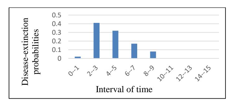
Figure 13 Disease extinction probabilities diagram for = 0.8.
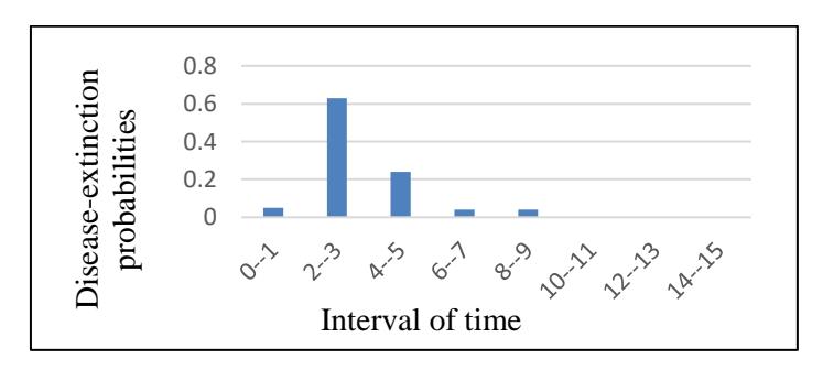
Figure 14 Disease extinction probabilities diagram for = 1.
Based on the simulation in Figures 9-14, the expected time until disease extinction was obtained as follows:
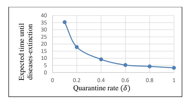
Figure 15 Graph of the effect of the quarantine rate on the expected time until disease extinction.
Figure 15 shows that for = 0.1, = 0.2, = 0.4, = 0.6, = 0.8, and = 1, the expected time until disease extinction was 35.34, 17.86, 9.22, 5.261, 4.277, and 3.284, respectively. The results of calculating the basic reproduction number (0 ), the expected number of infected individuals (), and the outbreak probability are presented in Table 5.
Table 5 Influence of on basic reproduction number, expected number of infected individuals, and outbreak probability.
| Value of Parameter 𝛿 | Basic reproduction number (𝑅𝑜) | Expected number of infected individuals (𝑚) | Outbreak probability |
|---|---|---|---|
| 0.1 | 1.341282 | 0.968486 | 0 |
| 0.2 | 1.096224 | 0.868367 | 0 |
| 0.4 | 0.802855 | 0.719589 | 0 |
| 0.6 | 0.633357 | 0.614334 | 0 |
| 0.8 | 0.522952 | 0.535942 | 0 |
| 1 | 0.445324 | 0.475292 | 0 |
Based on Table 5 it can be seen that for = 0.1, = 0.2, = 0.4, = 0.6, = 0.8 and = 1 an expected number of infected individuals () < 1 was obtained, which caused the value of outbreak probability to be 0 in each case. This means that when the quarantine rate is given in the system, if the number of infected individuals is decreasing then stochastically there will be no outbreak in the long-term. The outbreak probability is determined from the expected number of infected individuals () and not from the basic reproduction number (0 ). Because of this, although 0 > 1 for = 0.1, and = 0.2, also < 1 is obtained, which makes the outbreak probability 0.
In this study we did not focus on a comparison between stochastic and deterministic models. Especially for quarantine rate 0.1 and 0.2, the values of 0 > 1 and < 1 indicate that disease extinction will happen in the long run after an outbreak in a certain period. This means that even though a deterministic model shows an outbreak in the long term, it can be stochastically determined, because when the quarantine rate is 0.1 and 0.2 tuberculosis can disappear and there will be no outbreak in the long term.
The stochastic result can be different from the deterministic result because it considers the random effects of uncertain cases. The stochastic model uses random variables such as S (susceptible), I (infected), and Q (quarantined), which can change every time so there are probabilities in each case. Especially random variable I, the number of infected individuals, is probable to increase and decrease. Based on the branching process approach, for quarantine rate = 0.1 and = 0.2, the probability of a decreasing number of infected individuals is 0.5157 and 0.5658, respectively, so the probability of an increasing number of infected individuals is 0.4842 and 0.4341. Stochastically this indicates that there is a chance of < 1 and the disease will become extinct so there will be no outbreak in the long term.
Based on the simulation and analytical calculations it can be concluded that increasing the quarantine rate from = 0.1 to = 1 decreases the expected time until disease extinction, the basic reproduction number (0 ) and the expected number of infected individuals (), because of which < 1. This indicates that increasing the quarantine rate makes the disease disappear more rapidly from the population and reduces the contact between infected individuals and non-infected individuals so there will be no outbreak in the long term.
4.4 Sensitivity Analysis
A sensitivity analysis was performed to examine the effect of varying the parameter values in the model. The sensitivity index of 0 may be alternatively defined using partial derivatives as follows:
\[\Upsilon_p^{R_0} = \frac{\partial R_0}{\partial p} \times \frac{p}{R_0} \tag{9}\] where is the parameter value in the model. The sensitivity index can show the effect of relative changes of basic reproduction number 0 when the value of is changed [15]. A positive sensitivity index indicates that every increase of the number of units will increase 0 to |ϒ 0 | [16]. Based on Equation (9) and the parameter value of the simulation when 0 > 1, it is obtained that the sensitivity index of 0 is as follows:
| Parameters | 𝑅0 Sensitivity Index (ϒ𝑝 ) |
|---|---|
| 𝛽 | 1 |
| 𝜀 | – 0.7451 |
| 𝜇 | – 0.0313 |
| 𝛿 | – 0.2235 |
| 𝜆 | 0 |
| 𝛼 | 0 |
| 𝛾 | 0 |
Table 6 Sensitivity index of 0 .
Based on Table 6, it can be concluded that is a sensitive parameter towards 0. This is in accordance with the stochastic results in Tables 3, 4 and 5, where the transmission rate () has a larger influence on the expected number of infected individuals () than the other parameters.
5 Conclusion
It can be concluded that the SIQRS model can be used to determine the characteristics of the spread of infectious diseases such as tuberculosis. In stochastic models, an outbreak occurs when the expected number of infected individuals () > 1, whereas it does not occur when < 1. Based on the simulation of Scenario 1, the expected number of infected individuals () for = (365/365), = (365/730), and = (365/1095) was 0.002758, 0.005433, and 0.008029, respectively, where < 1. This indicates that an outbreak does not occur when the healing rate is decreasing, but it needs a long of time for the disease to disappear from the population.
In Scenario 2, the expected number of infected individuals () for = 0.2, = 0.4, and = 0.6 was 0.574555, 0.892667, and 1.0947, respectively. This indicates that an increase of the transmission rate can increase the expected number of infected individuals (), which leads to an outbreak in the long term. On the other hand, the simulation repeated 100 times with Scenario 3 showed that for = 0.1, = 0.2, = 0.4, = 0.6, = 0.8, and = 1, the expected time until disease extinction was 35.34, 17.86, 9.22, 5.261, 4.277, and 3.284, respectively, and the expected number of infected individuals () was 0.968486, 0.868367, 0.719589, 0.614334, 0.535942, and 0.475292, respectively, where < 1.
It can be concluded that an increase of the quarantine rate decreases the expected time until disease extinction and reduces the contact between infected individuals and non-infected individuals. It also makes the disease disappear more rapidly from the population so there will not be an outbreak in the long term. In general, the transmission rate is the most sensitive parameter in this system towards the occurrence of outbreaks.