1 Introduction

All graphs considered in this paper are connected, simple, undirected and finite. Let G(V, E) be a graph with vertex set V and edge set E. Let d(u, v) denote the distance between the vertices u and v. Let N[v] denote the closed neighborhood of the vertex \(v \in V\), i.e. \(N[v] = \{x \in V : d(x, v) \leq 1\}\). A neighborhood set of G is a subset S of the vertex set of G with the property that \(G = \bigcup_{v \in S} G_v\) where \(G_x = \langle N[x] \rangle\). Further, a subset S of V is called a resolving set of G if for each pair u, v of vertices of G there is a vertex \(t \in S\) with the property that |d(v,t)-d(u,t)|>0. A neighboring set of G that also serves as an F-set of G is called a neighborhood resolving set (nF-set) of G. In other words, an nF-set S is an ordered subset \(S=(s_1,s_2,s_3,...,s_k)\) of V such that \(F(x/S) \neq F(y/S)\) for all \(x,y \in V - S\) and \(G = \bigcup_{i=1}^k \langle N[s_i] \rangle\), where \(F(a/S) = (d(a,s_1), d(a,s_2), ..., d(a,s_k))\) is called the code of vertex E0 with respect to E1.

An nr-set is called a minimal nr-set (mnr-set) if none of its proper subsets is an nr-set. The mnr-set of G with least cardinality is called the neighborhood metric basis (nmb) and its cardinality is called the lower neighborhood metric dimension or simply the neighborhood metric dimension of graph G, denoted by nmd(G). Similarly, the upper neighborhood metric dimension of G is the greatest cardinality of an mnr-set, denoted by Nmd(G). Further, an nr-set S is called a maximal neighborhood resolving set (Mnr-set) whenever V-S is not an nr-set. The minimum cardinality of an Mnr-set is called the lower maximal neighborhood metric dimension or simply the maximal neighborhood metric dimension of G, denoted by nMd(G). Similarly, the maximum cardinality of an Mnr-set of G is called the upper maximal neighborhood metric dimension of G, denoted by NMd(G). These sets and dimensions have been studied for paths and cycles in [1]. Related work can be found in [2-19]. For the terms not defined here we refer to [20,22].

We recall the following theorem in [23]:

Theorem 1.1. Let G(V, E) be a graph and \(S \subseteq V(G)\). Then, S is an n-set of G if and only if every pair of adjacent vertices in \(\overline{S}\) is dominated by a common vertex in S [23].

Corollary 1.2. Let G be a triangle free graph. Then, S is an n-set of G if and only if \(\langle \bar{S} \rangle \equiv \overline{K}_n\), where \(\bar{S} = V(G) - S\) and n = |V(G)| [23].

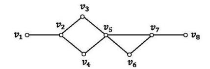
Figure 1 Graph G.

Example: The sets \(\{v_3, v_7\}\), \(\{v_2, v_5, v_7\}\), and \(\{v_2, v_3, v_5, v_8\}\) are an r-set, n-set, and nr-set of graph G in Fig. 1, respectively. The set \(\{v_2, v_3, v_4, v_7\}\) is a minimal nr-set.

Theorem 1.3. The minimum cardinality of an r-set of G is 1 if and only if \(G = P_n\) for some \(n \ge 2\) [24].

Theorem 1.4. Let T = (V, E) be a tree with \(\delta(T) \ge 3\). Then the minimum cardinality of an r-set is given by \(\sum_{v \in V: l_v > 1} (l_v - 1)\) [24].

Theorem 1.5. For any positive integer \[n\], \(nmd(P_n) = \begin{cases} \left\lceil \frac{n}{2} \right\rceil, & \text{if } n \leq 3 \\ \left\lfloor \frac{n}{2} \right\rfloor, & \text{if } n \geq 4 \end{cases}\) [1].

Remark 1.6. If graph G contains k pendent vertices adjacent to a vertex v in it, then every resolving set of G should contain at least k-1 of these pendent

vertices. Otherwise, two of these pendent vertices not in a resolving set receive the same code due to the fact that is a cut vertex.

We state the following theorems whose proof follows immediately from the definition of an -set and Theorem 1.3.

Theorem 1.7. For a connected graph , () = 1 if and only if ≃ ¹ 2.

Theorem 1.8. For any connected graph , 2 ≤ () ≤ |()| − 1, whenever |()| ≥ 3.

The upper bound in Theorem 1.8 is tight for the complete graph on vertices. In a later section of this paper we characterize the graphs that satisfy the lower bound and construct a graph of prescribed neighborhood dimension.

2 Application of Neighborhood Resolving Sets

In most safeguard applications of a network model, various types of protection sets have been studied to identify or locate an 'intruder' or to check a faulty processor. The locating sets are such a protection sets, not only to identify intruders but also to determine the distance to an intruder. These were introduced by Slater [25] and independently by Harary and Melter [26]. When two intruders are linked (known to each), then it is more efficient to have a common protection device at a vertex adjacent (known to) both intruders. However, the study of special types of dominating sets, namely neighborhood sets, was introduced in [23]. The neighborhood set is a notion that is somehow in between vertex cover and dominating sets. These sets are considered in [1] to build a powerful locating-dominating set, as they have the additional property of edge covering along with the domination and locating properties. Such sets are useful in the study of the location of vertices as well as edges in a network.

3 Realization

In this section we construct a graph with prescribed parameters.

Theorem 3.1. For the given positive integers , , with , ≤ , there is a tree on vertices such that () = , () = and () = whenever 2 − ≤ ≤ + .

Proof. Let () = , () = and () = . Then ≤ , ≤ and + ≥ . Let = + − ; ¹ = ̅− and ² = ( + − ) 2.

Consider a path 2(−) : ¹ − ² − … − 2(−) . Add the edges between one end vertex of each copy of ² in ² to the vertex 1, and each vertex of ¹ to 1. The graph thus obtained satisfies:

1) \[l_n(G) = \alpha\].

In fact, if is any -set, then should include ( − ) vertices of 2(−) and + − vertices of 2, because is triangular free and by Corollary 1.1, 〈 − 〉 is totally disconnected and hence || ≥ ( − ) + ( + − ) = .

On the other hand, the set = { , : is a vertex in the ℎ copy of ² in 2, ∈ ( 2(−)) and is odd } is an -set of with |S|≤ .

\[2) l_r(G) = \beta.\]

Since is a tree with + 1 legs it follows from Theorem 1.5 that () = + 1 − 1 = .

3) \[l_{nr}(G) = \gamma\].

Let be an -set of , then at least pendent vertices of should be in being an -set and − vertices of a path 2(−)() = being an -set. So || ≥ + − = .

On the other hand, = { : ∈ (2(−))} ∪ {: is a pendant vertex of not in } is an -set with || = .

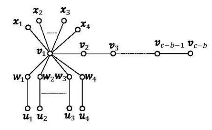
Figure 2 A tree G with () = , () = and () = .

As an immediate consequence of Theorem 3.1, we have:

Corollary 3.2. For the positive integers , , with , ≤ ≤ + there is a graph G, see Fig. 2, with () = , () = and () = .

4 Graphs of Neighborhood Metric Dimension Two

We begin this section with the following lemma:

Lemma 4.1. Let G be a connected graph and \(S = \{s_1, s_2\}\) be an independent nr-set of G. Then there is a unique vertex v that is adjacent to both \(s_1\) and \(s_2\) in G.

Proof. We first prove the existence. Since G is connected and S is an independent n-set, \(s_1\) is adjacent v, and \(s_2\) is adjacent to u for some \(u, v \in V(G)\). The vertex v does not need to be distinct from u. If v = u, then v is the desired vertex. Else, if u and v are distinct, then there is a vertex \(w_1 \in V(G) - S\) such that \(w_1\) is in the shortest path from v to u adjacent to v. But then, for the edge \(vw_1\), by Theorem 1.1 we see that \(w_1\) is adjacent to \(s_1\). If \(w_1\) is adjacent to \(s_2\), then \(w_1\) is the desired vertex. Otherwise, repeating this argument by replacing v with \(w_1\), we arrive at v finite steps that there is a vertex v desired vertex. Else, if v is not adjacent to v for any v, then for the last possible v we see that v is not adjacent to v for any v, then for the last possible v we see that v is adjacent to v is adjacent to v is adjacent to v is adjacent to v is adjacent to v is adjacent to v is adjacent to v is adjacent to v is adjacent to v is adjacent to v is adjacent to v is adjacent to v is adjacent to v is adjacent to v is adjacent to v is adjacent to v is adjacent to v is adjacent to v is adjacent to v is adjacent to v is adjacent to v is adjacent to v is adjacent to v is adjacent to v is adjacent to v is adjacent to v is adjacent to v is adjacent to v is adjacent to v is adjacent to v is adjacent to v is adjacent to v is adjacent to v is adjacent to v is adjacent to v is adjacent to v is adjacent to v is adjacent to v is adjacent to v is adjacent to v is adjacent to v is adjacent to v is adjacent to v is adjacent to v is adjacent to v is adjacent to v is adjacent to v is adjacent to v is adjacent to v is adjacent to v is adjacent to v is adjacent to v is adjacent to v is adjacent to v is adjacent to v is adjacent to v is adjacent to v is adjacent to v is adjacent to v is adjacent to v is adjacent to v

To prove uniqueness: Suppose that \(v_1\) and \(v_2\) are two distinct vertices adjacent to both \(s_1\) and \(s_2\). However, then \(d(v_1, s_1) = d(v_2, s_1)\) and \(d(v_1, s_2) = d(v_2, s_2)\) imply that S has no vertex that resolves \(v_1\) and \(v_2\), a contradiction (:S is an r-set).

Remark 4.2. If S is a non-independent nr-set, then G does not need to have a common vertex adjacent to both elements in S as in Lemma 4.1. Thus, S can have at most one vertex in V(G) - S that is adjacent to both \(s_1\) and \(s_2\) for any general nr-set S of cardinality 2.

Lemma 4.3. Let G be a connected graph and \(S = \{s_1, s_2\}\) be an nr-set of G. Then, \(1 \le deg(s_i) \le 3\), for each i = 1, 2.

Proof. Let us assume to contrary that \(deg(s_i) \ge 4\) for some i = 1,2. Without loss of generality we take \(deg(s_1) \ge 4\). Let \(v_1, v_2, v_3, v_4\) be the vertices adjacent to \(s_1\). Then:

Case 1: \(\langle S \rangle\) is independent.

In this case, by Lemma 4.1, there is a unique vertex x adjacent to both \(s_1\) and \(s_2\), and hence at least three of the vertices in \(\{v_1, v_2, v_3, v_4\}\) are not adjacent to \(s_2\). Without loss of generality, let \(v_1, v_2, v_3\) be the vertices not adjacent to \(s_2\).

But then, \(d(v_i, s_1) = 1\) and \(d(v_i, s_2) = \begin{cases} 3 & \text{if } v_i \ x \notin E(G) \\ 2 & \text{if } v_i \ x \in E(G) \end{cases}\). In either of these cases there are at least two vertices \(v_l, v_m \in \{v_1, v_2, v_3\}\) that satisfy \(d(v_l, s_2) = d(v_m, s_2)\), a contradiction to the fact that S resolves G. Case \(2: \langle S \rangle\) is connected.

In this case there are at least three vertices \(v_1, v_2, v_3\) not in S adjacent to \(s_1\) in G. But then, by Remark 4.2, at least two of these, say \(v_1\) and \(v_2\), are not adjacent to \(s_2\). So, \(d(v_1, s_1) = d(v_2, s_1)\) and \(d(v_1, s_2) = d(v_2, s_2) = 2\), a contradiction to the fact that S resolves G.

The above Lemma 4.1 and Lemma 4.3, together with the domination property of n-sets, yield the following theorem:

Lemma 4.4. If G is a connected graph of order n with nmd(G) = 2, then \(3 \le n \le 7\).

Lemma 4.5. Let G be a connected graph and \(S = \{s_1, s_2\}\) be the neighborhood metric basis of G. Let x be the vertex adjacent to both \(s_1, s_2\). If u, v are vertices adjacent to \(s_1\), then either u is adjacent to x or v is adjacent to x in G.

Proof. If not, then there are two possible cases: (i) both u and v are not adjacent to x, and (ii) both u and v are adjacent to x. By Lemma 4.1, neither u nor v is adjacent to \(s_2\). So, \(\Gamma(u/S) = \Gamma(v/S) = (1,3)\) and \(\Gamma\left(\frac{v}{s}\right) = \Gamma\left(\frac{u}{s}\right) = (1,2)\) in the cases (i) and (ii) respectively, a contradiction to the fact that S is an r-set.

Lemma 4.6. If G is a connected graph of size m and nmd(G) = 2, then \(2 \le m \le 10\).

Proof. Let nmd(G) = 2 and \(S = \{s_1, s_2\}\) be the neighborhood metric basis of G. The lower bound is trivial, as \(nmd(K_2) = 1\). To prove the upper bound, let \(s_{l,i}\) be the \(i^{th}\) vertex adjacent to \(s_1\) and \(s_{2,j}\) be the \(j^{th}\) vertex adjacent to \(s_2\). Then \(1 \le i, j \le 3\) (by Lemma 4.3), \(s_{1,i} = s_{2,j}\) for exactly one (i,j) (by Lemma 4.1) and \(s_{1,i}\) is adjacent to \(s_{1,1}\) for exactly one \(i, i \ge 2\) (by Lemma 4.5). Without loss of generality we take \(s_{1,1} = s_{2,1}\) as the common vertex adjacent to both \(s_1\) and \(s_2\). Similarly, \(s_{2,j}\) is adjacent to \(s_{1,1}\) for exactly one \(j, j, \ge 2\). Without loss of generality, we assume that \(s_{1,2}\) is adjacent to \(s_{1,1}\), \(s_{2,2}\) is adjacent to \(s_{2,1}\) (note that \(s_{1,1} = s_{2,1}\)). Further, by Lemma 4.4, \(s_1\) has at most \(s_2\), \(s_1\), \(s_2\), \(s_2\), for \(s_2\) for \(s_1\) deg \(s_2\). Therefore, \(s_2\) deg \(s_2\) deg \(s_3\)

\[\sum_{i=2}^{3} \deg(s_{1,i}) + \sum_{j=2}^{3} \deg(s_{2,j}) + \deg(s_{1,1}) \le (3+3) + (3+2) + (3+2) + 4 = 20. \text{ Hence, } m = \frac{1}{2} \sum_{v \in V} \deg(v) \le \frac{1}{2} (20) = 10.\]

Lemma 4.7. A graph G with nmd(G) = 2 cannot have an induced cycle \(C_n\) for any \(n \ge 4\).

Proof. Suppose to contrary that nmd(G)=2 and G has an induced cycle \(C_n\) for some \(n \ge 4\). Then \(C_n\) has no induced triangle. Let \(S = \{s_1, s_2\}\) be the neighborhood metric basis for G. We have only the following three cases:

Case (1): \[s_1, s_2 \in V(C_n)\]

In this case, S is not an independent set (by Lemma 4.1). Since \(n \geq 4\), there is an edge \(uv \in \langle V(C_n) - S \rangle\). However, then by Theorem 1.1 either \(\langle \{u, v, s_1\} \rangle\) or \(\langle \{u, v, s_2\} \rangle\) is an induced triangle of \(C_n\), a contradiction to the fact that \(C_n\) has no induced triangle.

Case (2): \[s_1 \in V(C_n)\] and \(s_2 \notin V(C_n)\)

Let x and u be the vertices of \(C_n\) adjacent to \(s_1\). By Lemma 4.1 the vertex \(s_2\) can be adjacent to at most one of these vertices, say \(u \notin N(s_2)\). Then, by Theorem 1.1, the vertex \(u'(\neq s_1)\) adjacent to u in \(C_n\) should be in \(N(s_1)\) and hence \((\{s_1, u, u'\})\) is an induced triangle of \(C_n\), a contradiction.

Case (3): \[s_1, s_2 \notin V(C_n)\]

In this case, by Lemma 4.5, n=4 or n=5. By Lemma 4.1, \(s_1\) and \(s_2\) are adjacent to at most one common vertex \(x \in V-S\). Therefore, there exist two adjacent vertices \(u,v \in V(C_n)\) such that \(u,v \notin N(s_1) \cap N(s_2)\). In view of Theorem 1.1, without loss of generality we take \(u,v \notin N(s_1)\) (hence \(u,v \in N(s_2)\)). Since \(n \geq 4\), there are two distinct vertices u' and v'adjacent to respectively u and v in \(C_n\). Let \(v' = x \in N(s_1) \cap N(s_2)\) and from Remark 4.2 \(s_1\) is adjacent to only u'. Then an edge \(uu' \notin \bigcup_{v \in S} \langle N[v] \rangle\), a contradiction to an n-set S. And also \(\Gamma(u/S) = \Gamma(v/S) = (1,2)\) implies S is not an r-set.

Lemma 4.8. A graph G with nmd(G) = 2 cannot have an induced subgraph isomorphic to \(P_6\).

Proof. Let nmd(G) = 2 and S be any nmb of G. If possible, let \(P_6\): \(v_1\), \(v_2\), ..., \(v_6\) be an induced path of G with \(v_iv_{i+1} \in E\) for each i, \(1 \le i \le 5\). If G has no other vertices, then \(G \cong P_6\), a contradiction to the fact that \(nmd(P_6) = 3\) (by Theorem 1.5). Further, as G can have at most 7 vertices (by Lemma 4.4),

G has exactly one new vertex v. The graph \(G \not\simeq P_7\) (since \(nmd(P_7) = 3 > 2\), by Theorem 1.5) and hence v cannot be adjacent to only \(v_1\) or only \(v_6\). Also, if v is not adjacent to both \(v_1\) and \(v_6\), then by Theorem 1.1, every nmr-set S should include at least two vertices from the set \(\{v_1, v_2, v_5, v_6\}\) for the edges \(v_1v_2\) and \(v_5v_6\), and a new vertex for the edge \(v_3v_4\), so \(|S| \ge 3 \Rightarrow nmd(G) \ge 3\), a contradiction. Finally if v should be adjacent to both \(v_1\) and \(v_6\), then by Lemma 4.7, the vertex v is adjacent to every \(v_i\), \(2 \le i \le 5\) and hence G has 11 edges, a contradiction by Lemma 4.6. Thus, v should be adjacent to exactly \(v_1\) (or \(v_6\) but not both) and a vertex \(v_i\), \(0 \le i \le 5\). Without loss of generality we assume \(v_1 \in E\).

If \(v \notin S\), then by Theorem 1.1 for the edge \(vv_1\), either \(v_1 \in S\), or \(v_2 \in S\) and \(vv_2 \in E(G)\). Let \(S = \{v_i, v_j\}\) where i = 1 or i = 2, and \(i + 1 \le j \le 5\). Then by Lemma 4.7, we get j = i + 1. But then for the edge \(v_5v_6\), by Theorem 1.1, either \(v_i\) or \(v_{i+1}\) adjacent to both \(v_5\) and \(v_6\), a contradiction to the fact that \(P_6\) is an induced path. Therefore, \(v \in S\) and hence \(S = \{v, v_1\}\). But then, again for the edge \(v_5v_6\), by Theorem 1.1 only v should be adjacent to both \(v_5\) and \(v_6\) (since \(P_6\) is an induced path), a contraction to the fact that v is not adjacent to \(v_6\). Hence the theorem is proved.

Lemma 4.9. Let G be a graph of order n and S be a neighborhood metric basis of cardinality 2 in G. If S has a pendent vertex of G, then \(n \le 5\).

Proof. Let \(S = \{s_1, s_2\}\) be the neighborhood metric basis and \(s_1\) be a pendent vertex in S. If \(s_2\) is adjacent to \(s_1\), then \(d(s_1, x) = d(s_2, x)\) for every \(x \in V(G)\) and hence \(s_2\) may be adjacent to at most one more vertex in G, which implies that \(n \leq 3\). If \(s_2\) is not adjacent to \(s_1\), then S is an independent set. Hence by Lemma 4.1, G has exactly one vertex adjacent to both \(s_1\) and \(s_2\). Finally, as each vertex of G is adjacent to either \(s_1\) or \(s_2\), the order of \(G = |N[s_1] \cup N[s_2]| = |N[s_1]| + |N[s_2]| - |N[s_1] \cap N[s_2]| = 2 + 4 - 1 = 5\).

Lemma 4.10. A graph G with nmd(G) = 2 cannot have a subgraph isomorphic to \(K_4\).

Proof. Let nmd(G) = 2 and \(S = \{s_1, s_2\}\) be an nmr-set of G. If possible, suppose to contrary that G has a subgraph H isomorphic to \(K_4\). Let \(v_1, v_2, v_3, v_4\) be the vertices of H. Then we have the following cases:

Case (i): \(S \subseteq H\)

In this case, for the vertices, \(x, y \in H - S\), we get \(d(s_1, x) = d(s_2, x)\); \(d(s_1, y) = d(s_2, y) = 1\), a contradiction to the fact that S is an r-set.

Case (ii): \(|S \cap V(H)| = 1\).

Without loss of generality we take \(s_1 = v_1 \in S \cap V\), then in this case \(s_2 \neq v_i\), for any \(i, 2 \leq i \leq 4\) and \(s_1\) is adjacent to each \(v_j, 2 \leq j \leq 4\). Hence by Lemma 4.3, \(s_1\) is not adjacent to \(s_2\) as well no other vertex in V(G) - V(H). So, by Lemma 4.1, there is a vertex \(v_j\) for exactly one \(j, 2 \leq j \leq 4\), adjacent to both \(s_1\) and \(s_2\). Without loss of generality, we take \(v_2\) is adjacent to \(s_1\) and \(s_2\). But then, \(\Gamma(v_3|S) = \Gamma(v_4|S) = (1,2)\), a contradiction to the fact that S is an r-set.

Case (iii): \(|S \cap V(H)| = \emptyset\).

By Theorem 1.1, for the edge \(v_1v_2\), we have either \(v_1, v_2 \in N(s_1)\) or \(v_1, v_2 \in N(s_2)\). Without loss of generality we take \(v_1, v_2 \in N(s_1)\). By Lemma 4.3, \(s_1\) can be adjacent to at most one of the vertices in \(\{v_3, v_4\}\), and by Lemma 4.1, \(s_2\) can be adjacent to at most one vertices in \(\{v_1, v_2\}\). Without loss of generality, we take \(v_3 \notin N(s_1)\) and \(v_1 \notin N(s_2)\). However, then G has no triangle containing the edge \(v_1v_3\), one of its vertices in S, a contradiction (by Theorem 1.1) to the fact that S is an n-set.

Corollary 4.11. If S is a neighborhood metric basis of cardinality 2 of a graph G, then the graph \(\langle V - S \rangle\) is acyclic.

Proof. If not, then by Lemma 4.7, \(\langle V - S \rangle\) has a triangle. Let \(v_1, v_2, v_3\) be vertices in a cycle of \(\langle V - S \rangle\). Then, by Theorem 1.1 both end vertices of the edge \(v_1v_2\) are adjacent to one of the vertices in S, say \(s_1\). If \(v_3\) is adjacent to \(s_1\), then \(\langle \{v_1, v_2, v_3, s_1\} \rangle\) is an induced \(K_4\), a contradiction to Lemma 4.10. So, \(v_3\) is not adjacent to \(s_1\).

Now, by Theorem 1.1 the end vertices \(v_2, v_3\) of the edge \(v_2 v_3\) should be adjacent to \(s_2\). But then \(v_2\) is adjacent to both \(s_1\) and \(s_2\) and hence by Lemma 4.1, \(v_1\) cannot be adjacent to \(s_2\). Therefore none of the end vertices of edge \(v_1v_3\) are adjacent to \(s_1\) or \(s_2\), a contradiction to Theorem 1.1.

We now prove our main theorem of this section.

Theorem 4.12. For a graph G, the neighborhood metric dimension, nmd(G) = 2 if and only if G is isomorphic to one of the graphs in Fig. 3.

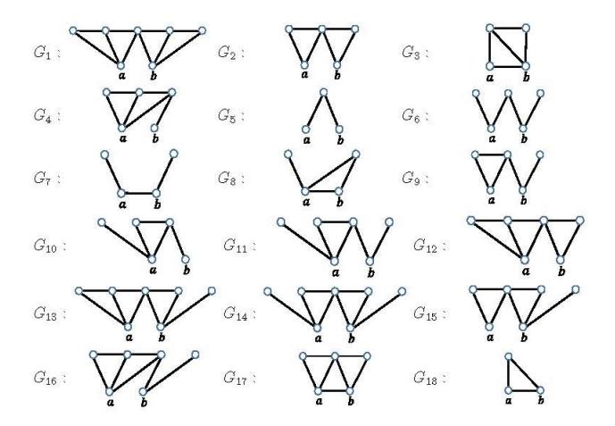
Figure 3 Graphs of neighborhood metric dimension two.

Proof. For the graphs 6, 7, and 5, an -set should contain a non-pendent vertex. But such a set with cardinality less than 2 is not a resolving set. Hence () ≥ 2. Other graphs in the Figure are not paths, hence by Theorem 1.3 it follows that () ≥ 2. The reverse inequality follows by noting that the set = {, } is an -set for each of the graphs.

Conversely, let be any connected graph with () = 2 and let S = {1, 2} be a neighborhood resolving basis of . Then, by Corollary 4.11 〈 − 〉 is a forest. Therefore we have only the following cases:

Case 1: 〈〉 is connected.

By Lemma 4.1 and Lemma 4.3, 〈 − 〉 has at most two edges.

Subcase 1: 〈 − 〉 ≃ ³ ∪ m1.

By Theorem 1.1 and Lemma 4.1, both end vertices of one of the edges of ³ should be adjacent to ¹ and both end vertices of other edges to 2. Therefore the center of ³ is adjacent to both ¹ and 2. Thus by Lemma 4.3, neither ¹ nor ² is adjacent to any more vertex, which implies that = 0. Hence ≃ ¹⁷ in this case.

Subcase 2: 〈 − 〉 ≃ 2² ∪ m1.

In this case both vertices of one of the copies of ² are adjacent to one of the vertices in , say 1, and both vertices of the other copy of ² should be adjacent to only \(s_2\). Further, by Lemma 4.3, m = 0. We observe that \(G \simeq P_2 \odot P_2\), so the end vertices in each copy of \(P_2\) receive the same code with respect to S. Therefore, no graph G exists with nmd(G) = 2 in this case.

Subcase 3: \(\langle V - S \rangle \simeq P_2 \cup mK_1\).

As above, \(P_2\) should be adjacent to one of the vertices in S, say \(s_1\). But then, by Lemma 4.3 the vertices of \(mK_1\) are adjacent to only \(s_2\) and \(m \le 2\). Further, none of these pendent vertices are in S and hence by Remark 1.6 it follows that \(m \ne 2\). Therefore \(m \le 1\).

If m = 0, then by Lemma 4.10, exactly one of the end vertices of \(P_2\) should be adjacent to \(s_2\) (else the end vertices of \(P_n\) receive the same code or induce \(K_4\)). Thus, \(G \simeq G_3\) in this case.

If m=1, then as above exactly one of the vertices of \(P_2\) should be adjacent to \(s_2\) (to resolve the vertices of \(P_2\)). Hence graph \(G \simeq G_4\) in this case.

Subcase 4: \(\langle V - S \rangle \simeq mK_1\).

In this case, one of the isolated vertices in \(\langle V - S \rangle\) may be common to both elements in S (by Lemma 4.1) and each vertex in S may be adjacent to at most one isolated vertex in G (by Remark 1.6). Therefore \(m \leq 3\) and \(G \simeq G_5\), \(G_7\), \(G_8\), \(G_{10}\), \(G_{18}\).

Case (ii): \(\langle S \rangle\) is disconnected.

In this case, in view of Lemma 4.1 and Lemma 4.3, the graph \(\langle V - S \rangle\) can have at most four edges.

Subcase (i): \(\langle V - S \rangle\) is totally disconnected.

Let \(\langle V - S \rangle = mK_1\). Then \(m \ge 1\), else G is disconnected. Suppose that \(u_1\), \(u_2\), ..., \(u_m\) are the vertices in \(\overline{K_m} = mK_1\). By Lemma 4.1, without loss of generality we take \(u_1\) is the only vertex that is adjacent to both \(s_1\) and \(s_2\).

If m = 1, then \(G \simeq G_5\) in this case.

If \(m \ge 2\), then \(u_2\) is adjacent to exactly one of the vertices in S, say \(s_1\). Now, \(G \simeq G_7\) if m = 2. Else if \(m \ge 3\), then by Remark 1.6 \(u_3\) is adjacent to only \(s_2\). Therefore \(G \simeq G_6\) if m = 3. Finally, if m > 3 then by the pigeonhole principle, at least one of the vertices in S is a support for at least two pendent vertices not in S. By Remark 1.6 no such graph with nmd(G) = 2 exists.

Subcase (ii): 〈 − 〉 has exactly one edge.

In this case, 〈 − 〉 ≃ ² ∪ ¹ and by Theorem 1.1 both vertices of ² are adjacent to exactly one of the vertices of , say 1. By Lemma 4.1 exactly one of the vertices of ² is adjacent to 2. Therefore, similar to Subcase (i) it follows that ≃ ⁸ if = 0; ≃ ⁹ or ¹⁰ if = 1; ≃ ¹¹ if = 2; and no graph exists if ≥ 3.

Subcase (iii): 〈 − 〉 has exactly two edges.

Subsubcase (i): 〈 − 〉 ≃ 2² ∪ m1.

In this case, since is an -set, both vertices of one of the copies of ² are adjacent to exactly one of the vertices in , say 1. Also exactly one of the vertices of this copy of ² is adjacent to 2. Similarly, both vertices of the other copies of ² are adjacent to only ² and exactly one of them is adjacent to 1. Hence there are two vertices, one from each copy of 2, that are adjacent to both ¹ and 2, which is not possible by Lemma 4.1. Therefore, no graph exists in this case with () = 2.

Subsubcase (ii): 〈 − 〉 ≃ ³ ∪ m1.

If all vertices of ³ are adjacent to a vertex in , say 1, then exactly one of the end vertices of ³ should be adjacent to ² (by Lemma 4.1) to resolve all vertices of ³ by 2. Further, no vertex of ¹ is adjacent to ¹ (by Lemma 4.3) and at most one vertex is adjacent to ² (by Remark 1.6). Therefore, ≤ 1, and ≃ ⁴ if = 0, and ≃ ¹⁶ if = 1.

If all vertices of ³ are not adjacent to a vertex in , then the end vertices of the edges are adjacent to ¹ and the end vertices of the other edges are adjacent to 2, and hence the central vertex of ³ is adjacent to both ¹ and 2. Further, by Lemma 4.1 and Remark 1.6 vertex ¹ may be adjacent to a pendent vertex of ¹ and ² may be adjacent to at most one other pendent vertex in of 1, which implies that ≤ 2. Hence ≃ ² if = 0; ≃ ¹⁵ if = 1; and ≃ ¹⁴ if = 2.

Subcase (iv): 〈 − 〉 has exactly three edges.

Subsubcase (i): 〈 − 〉 ≃ ⁴ ∪ m1.

Let 1, 2, 3, ⁴ be the vertices of 4. Then, as above, if the vertices 1, ² are adjacent to say 1, the vertices 3, ⁴ are adjacent to ² (by Theorem 1.1 and

Lemma 4.3). Further, for the edge \(v_2v_3\), by Theorem 1.1 either \(v_2\) is adjacent to \(s_2\), or \(v_3\) is adjacent to \(s_1\). Thus, similar to the previous arguments on \(mK_1\), \(G \simeq G_{12}\) if m = 0; \(G \simeq G_{13}\) if m = 1; and no graph exists if m > 1 (since \(deg(s_i) = 3\), for one i = 1, 2).

Subsubcase (ii): \(\langle V - S \rangle \simeq (P_3 \cup P_2) \cup mK_1\).

In this case, both the end vertices of \(P_2\) should be adjacent to one of the vertices of S say \(s_1\). But then by Theorem 1.1 and Lemma 4.3 all the vertices of \(P_3\) should be adjacent to \(s_2\), and by Lemma 4.1 exactly one of the end vertices of \(P_3\) should be adjacent to \(s_1\) (to resolve all the vertices of \(P_3\)). But then m = 0 (since already \(deg(s_1) = deg(s_2) = 3\)). Now, the end vertices of \(P_2\) are equidistant from \(s_1\) (at a distance 1) as well as equidistant from \(s_2\) (at a distance 2). Therefore, no graph G exists in this case with nmd(G) = 2.

Subsubcase (iii): \(\langle V - S \rangle \simeq 3P_2 \cup mK_1\).

In this case \(n \ge |S| + 3|P_2| + m \ge 2 + 6 + 0 = 8\). Hence, by Lemma 4.4, no graphs exist in this case.

Subcase (v): \(\langle V - S \rangle\) has exactly four edges.

By Lemma 4.3 the maximum number of vertices in \(\langle V - S \rangle\) is 5. Therefore the only the possible forests are \(\langle V - S \rangle \simeq\) a path \(P_5\) or a Bistar \(B_{1,2}\) or a star \(K_{1,4}\) or \((K_{1,3} + e) \cup mK_1\) with \(m \in \{0,1\}\).

Subsubcase (i): \(\langle V - S \rangle \simeq P_5\).

Let \(v_1\), \(v_2\), \(v_3\), \(v_4\), \(v_5\) be the vertices of \(P_5\). Then by Theorem 1.1, Lemma 4.1 and Lemma 4.3 the only possibility is that \(s_1\) is adjacent to \(v_1\), \(v_2\), \(v_3\), and \(s_2\) is adjacent to \(v_3\), \(v_4\), \(v_5\). The graph \(G \simeq G_1\) exists in this case.

Subsubcase (ii): \(\langle V - S \rangle \simeq B_{1,2}\).

Let \(v_1, v_2, v_3, v_4, v_5\) be the vertices of \(B_{1,2}\) and \(v_1v_2, v_2v_3, v_3v_4, v_3v_5\) be its edges. By Theorem 1.1 and without loss of generality we assume that \(v_3, v_5 \in N(s_2)\).

If \(v_3, v_4 \notin N(s_2)\), then by Theorem 1.1, \(v_3, v_4 \in N(s_1)\) and hence \(v_3\) is the vertex adjacent to both \(s_1\) and \(s_2\). So for the edge \(v_2v_3\), by Theorem 1.1 by symmetry, we assume that \(v_2 \in N(s_1)\). But then by Lemma 4.1 \(v_2 \notin N(s_2)\) and hence for the edge \(v_1v_2\) by Theorem 1.1 \(v_1 \in N(s_1)\), therefore \(deg(s_1) \geq 4\), a contradiction to Lemma 4.3. Thus, \(v_3, v_4 \in N(s_2)\), and \(v_3\) is adjacent to both \(s_1\) and \(s_2\). But then, \(\Gamma(v_4|S) = \Gamma(v_5|S) = (1,2)\), so S cannot be an r-set and hence there is no graph G with nmd(G) = 2 in this case.

Subsubcase (iii): \(\langle V - S \rangle \simeq K_{1.4}\).

Let v be the central vertex and \(v_1, v_2, v_3, v_4\) be the end vertices of \(K_{1,4}\). Then by Lemma 4.1, Lemma 4.3 and Theorem 1.1, without loss of generality we assume only the possibilities that \(\{v_1, v_2, v\} = N(s_1)\) and \(\{v_3, v_4, v\} = N(s_2)\). Now, for the vertices \(v_3, v_4\), we get \(\Gamma(v_3|S) = \Gamma(v_4|S) = (1,2)\), and hence S cannot be an r-set. Therefore, there is no graph G with nmd(G) = 2 in this case.

Subsubcase (iv): \(\langle V - S \rangle \simeq (K_{1,3} + e) \cup mK_1, \ 0 \le m \le 1\).

Let \(v_1, v_2, v_3, v_4\) be the vertices of \((K_{1,3} + e)\) and \(v_1v_2, v_1v_3, v_2v_3, v_3v_4\) be its edges. By Theorem 1.1 without loss of generality we assume that \(v_3, v_4 \in N(s_1)\). From Lemma 4.10, \(\{v_1, v_2, v_3\} \nsubseteq N(s_1)\). Without loss of generality we assume that \(v_1\) is adjacent to \(s_1\), and \(v_2\) is adjacent to \(s_2\). But then by Theorem 1.1, \(v_3 \in N(s_2)\) and hence by Lemma 4.1 \(v_4 \notin N(s_2)\). Thus, for the vertices \(v_1, v_4\), \(\Gamma(v_1/S) = \Gamma(v_4/S) = (1,2)\) implies that S cannot be an r-set. Therefore, there is no graph G with nmd(G) = 2 in this case. Hence the theorem is proved.

5 Conclusion and Open Problems

An NP-complete problem of uniquely determining the location of an intruder in a network was the principal motivation behind introducing the concept of metric dimension in graphs by P.J. Slater.

In many practical situations, the role of a vertex in a network depends on its neighborhood. Since every neighborhood set is a dominating set, the concept of the neighborhood resolving set can be related to connected dominating sets, which has wide applications in building algorithms for wireless sensor networks (WSNs). The common approach to constructing a backbone for a WSN is to build a set of nodes such that every other node is close to a node in the given set. Such a set is known as a dominating set. The concept of the nr-set studied in this paper not only covers neighboring nodes but also distinguishes them through their resolving property. The idea of connected nr-sets can also be used in ad-hoc networks. The main result of this paper is a nice characterization of graphs of nr-dimension two. In general, it is natural to ask for a characterization of graph classes with respect to the nature of their neighborhood metric dimension. Thus, we end this section with some open problems:

• 1. Find a vertex transitive graph (, ) of regularity with () = for every possible 2 ≤ ≤ || − 1.
• 2. Find an algorithm to execute a minimal (optimal) connected -set of a given connected graph (, ).
• 3. Solve the graph equation () = || − 1 for (, ).

Acknowledgments

The authors wish to express sincere thanks to the referees for their careful reading of the manuscript and helpful suggestions.