
1 Introduction
Malaria is an infectious disease that has a major impact on health, social networks and the economy, and is mostly found in tropical and subtropical countries. Based on estimates of the World Health Organization (WHO) there were 216 million cases of malaria in 2016, 217 million cases in 2017, and up to 219 million cases in 2018 [1,2]. The number of deaths due to this disease reached 445 thousand in 2016 and decreased to 434 thousand in 2017 and 2018. Children under 5 years of age are the most vulnerable to the disease. In 2017, nearly 61% of all deaths caused by malaria were among young children.
Malaria is caused by protozoa genera of Plasmodium i.e. Plasmodium falciparum, Plasmodium malariae, Plasmodium ovale, and Plasmodium vivax. Plasmodium falciparum is the most common cause of infection in South East Asia, Africa, and South America. It contributes 80% of all malaria cases, with 90% of them leading to death. During its life cycle, the protozoa live in two
type of hosts: vector female Anopheles mosquitoes and humans. They grow rapidly in the human blood [3].
Mathematical models are intended to simplify the phenomenon of disease transmission between humans and mosquitoes using relevant clinic and biological information. There are two major types of models for infectious diseases: deterministic and stochastic models. There have been many related studies on host-vector transmission using either deterministic or stochastic models [4-9].
The first mathematical model of malaria disease transmission was introduced by Ross [10] using a deterministic differential equation by grouping the human population into \(S_h\) (susceptible) and \(I_h\) (infected), while the mosquito population is grouped into \(S_v\) (susceptible) and \(I_v\) (infected). Macdonald [11] expanded the model by adding a latent period for the mosquito population and the \(E_v\) group (exposed mosquitoes). Furthermore, Kingsolver [12] modeled malaria disease spread by taking into account manipulation by the malaria parasite. Accordingly, in Lacroix et al. [13], the malaria parasite manipulates the host to be more attractive to mosquitos through chemical substances.
In the present study, an SIS-SI model of the spread of malaria, developed by Chamchod & Britton [14], was further modified by including the attractiveness of mosquitos to hosts, formulated by a deterministic model. Also, the model was formulated within a stochastic framework, considering the human immunity factor related to malaria. The stochastic model is carried out using the continuous time Markov chain (CTMC) approach. In addition, the transition probability, the outbreak probability, the expected time required to reach a disease-free equilibrium, and the quasi-stationary probability distribution were calculated. In the last part of this work, a numerical simulation was conducted to analyze the behavior of malaria spread in several given conditions.
2 Mathematical Model
In this study, the model developed by Chamchod & Britton [14] was intensively investigated. The total human population, denoted by \(N_h(t)\), is grouped into two compartments, \(S_h(t)\) and \(I_h(t)\). The total population of mosquitoes, denoted by \(N_v(t)\), is also categorized into two compartments, \(S_v(t)\) and \(I_v(t)\). Infected humans may recover following treatment, but some of them may return to the susceptible compartment. Meanwhile, infected mosquitoes cannot recover. In the model, it is assumed that the parasite can manipulate the host to make itself more attractive to so that mosquitoes will be more interested in biting infected humans. In addition, Mading and Yunarko in [15] state that humans can have immunity to malaria, which can arise naturally or through
vaccination. Chamchod and Britton's model was modified by adding the assumption of immunity, so that not all susceptible humans bitten by infected mosquitoes are infected. A flow diagram of the model is shown in Fig. 1.
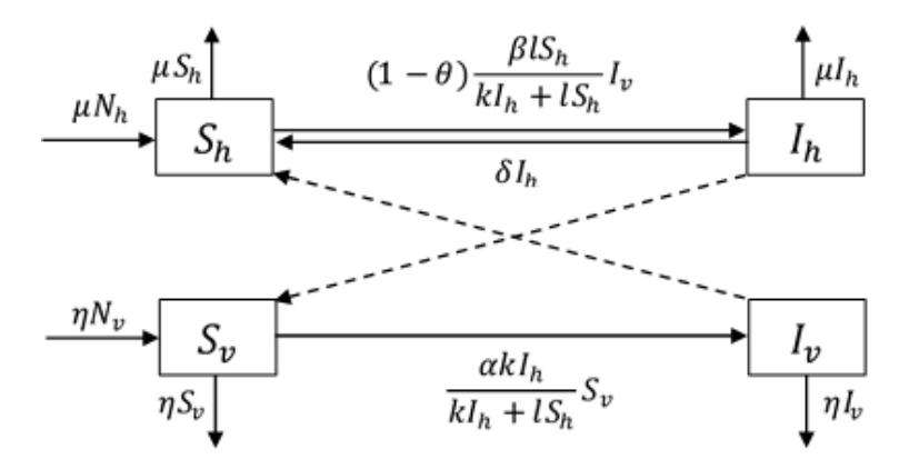
Figure 1 Compartmental diagram of the SIS-SI type model of malaria disease spread.
Based on the diagram above, we obtain the following system of ordinary differential equations:
\[\frac{dS_h}{dt} = \mu N_h - (1 - \theta) \frac{\beta l S_h}{k I_h + l S_h} I_v - \mu S_h + \delta I_h\] \[\frac{dI_h}{dt} = (1 - \theta) \frac{\beta l S_h}{k I_h + l S_h} I_v - (\mu + \delta) I_h\] \[\frac{dS_v}{dt} = \eta N_v - \frac{\alpha k I_h}{k I_h + l S_h} S_v - \eta S_v\] \[\frac{dI_v}{dt} = \frac{\alpha k I_h}{k I_h + l S_h} S_v - \eta I_v.\] (1)
The definitions of the parameters used in the model are listed in Table 1.
3 CTMC Stochastic Model
In this section, we will determine the transition probability, the outbreak probability, the expected time required to reach a disease-free equilibrium, and the quasi-stationary probability distribution for the SIS-SI model mentioned above.
| Parameter | Description | Value | Reference | |
|---|---|---|---|---|
| \(\overline{N_h}\) | Total population of humans | varied | - | |
| \(N_v\) | Total population of mosquitoes | varied | - | |
| \(\mu\) | Birth or death rate of humans | 1/70 (year -1) | [14] | |
| \(\eta\) | Birth or death rate of mosquitoes | 365/20 (year -1) | [16] | |
| δ | Recovery rate | 365/180 (year -1) | [17] | |
| β | Transmission rate in humans | 10 (year -1) | [18] | |
| α | Transmission rate in mosquitoes | 30 (year -1) | [18] | |
| k | Probability that a mosquito bites an infectious human | 0 - 1 | - | |
| l | Probability that a mosquito bites a susceptible human \((k > l)\) | 0 - 1 | - | |
| \(\theta\) | Effectiveness of the human immunity system | 0 - 1 | - | |
Table 1 Model parameters.
3.1 Transition Probability
The transition probability is the probability that a process originally in state i transitions to state j after a certain time has elapsed. This model is a bivariate process consisting of two random variables \(I_h\) and \(I_v\), where \(S_h = N_h - I_h\) and \(S_v = N_v - I_v\). It is assumed that the following Markov properties are satisfied:
\[P\{I_{h}(t + \Delta t), I_{v}(t + \Delta t) | (I_{h}(0), I_{v}(0)), (I_{h}(\Delta t), I_{v}(\Delta t)), \dots, (I_{h}(t), I_{v}(t))\} = P\{I_{h}(t + \Delta t), I_{v}(t + \Delta t) | I_{h}(t), I_{v}(t)\}.\]
Suppose \(I_h(t) = i_h\), \(I_v(t) = i_v\), \(I_h(t + \Delta t) = j_h\) and \(I_v(t + \Delta t) = j_v\), where \(i_h, j_h = 0, 1, ..., N_h\) and \(i_v, j_v = 0, 1, ..., N_v\). The transition probability that originates from state \((i_h, i_v)\) and transitions to state \((j_h, j_v)\) can be expressed as follows:
\[p_{(j_h, j_v), (i_h, i_v)}(t, t + \Delta t) =\] \[P\{I_h(t + \Delta t) = j_h, I_v(t + \Delta t) = j_v | I_h(t) = i_h, I_v(t) = i_v\}.\]
Based on the model transition probability it is assumed that \(\Delta t\) is sufficiently small so that during this tiny time interval only at most one single transition event exists for a particular random variable. The transition probabilities in this model are formulated as follows:
\[\begin{split} p_{(j_h,j_v),(i_h,i_v)}(t,t+\Delta t) \\ &= \begin{cases} (1-\theta)\frac{\beta l(N_h-i_h)}{ki_h+l(N_h-i_h)}i_v\Delta t + o(\Delta t), & (j_h,j_v) = (i_h+1,i_v) \\ (\delta+\mu)i_h\Delta t + o(\Delta t), & (j_h,j_v) = (i_h-1,i_v) \\ \frac{\alpha ki_h}{ki_h+l(N_h-i_h)}(N_v-i_v)\Delta t + o(\Delta t), & (j_h,j_v) = (i_h,i_v+1) \\ \eta i_v\Delta t + o(\Delta t), & (j_h,j_v) = (i_h,i_v-1) \\ (1-\omega(i_h,i_v))\Delta t + o(\Delta t), & (j_h,j_v) = (i_h,i_v) \\ o(\Delta t), & \text{otherwise} \end{cases} \end{split}\] where
\[\omega(i_h, i_v) = (1 - \theta) \frac{\beta l(N_h - i_h)}{k i_h + l(N_h - i_h)} i_v + (\delta + \mu) i_h + \frac{\alpha k i_h}{k i_h + l(N_h - i_h)} (N_v - i_v) + \eta i_v.\]
3.2 Derivation of Probability of Malaria Disease Outbreak
An outbreak event occurs when the number of infected humans increases as time goes on. Allen & Lahodny [19] derived a stochastic threshold for disease extinction and outbreak probability by using the multiple branching process approach. In this method, outbreak probability is determined by using a probability generating function (pgf). Firstly, we assume that the initial values of \(N_h(0)\) and \(N_v(0)\) are sufficiently large and nearly the same. The offspring pgf of \(I_h\), given \(I_h(0) = 1\) and \(I_v(0) = 0\), is:
\[f_1(h_1, h_2) = \frac{(\mu + \delta) + \left(\frac{\alpha k}{l}h_1 h_2\right)}{\left((\mu + \delta) + \frac{\alpha k}{l}\right)}\]
And the offspring pgf of \(I_v\), given \(I_h(0) = 0\) and \(I_v(0) = 1\), is
\[f_2(h_1, h_2) = \frac{\eta + (1-\theta)\beta h_1 h_2}{(\eta + (1-\theta)\beta)}.\]
The fixed point of pgf is found by setting \(f_i(h_1, h_2) = h_i\), i = 1,2, and solving for \(h_i\). So that, we have
\[h_1 = -\frac{l(\beta + \eta - \beta \theta)(\delta + \mu)}{\beta(-1 + \theta)(k\alpha + l(\delta + \mu))}\] and
\[h_2 = \frac{\eta(k\alpha + l(\delta + \mu))}{k\alpha(\beta + \eta - \beta\theta)}\] where \(0 < h_i < 1\). The expectation matrix of the offspring pfg evaluated at \((h_1, h_2) = (1,1)\) is given by
\[M = \begin{pmatrix} \frac{\partial f_1(h_1, h_2)}{\partial h_1} & \frac{\partial f_2(h_1, h_2)}{\partial h_1} \\ \frac{\partial f_1(h_1, h_2)}{\partial h_2} & \frac{\partial f_2(h_1, h_2)}{\partial h_2} \end{pmatrix} = \begin{pmatrix} \frac{\alpha k}{l \left( (\mu + \delta) + \frac{\alpha k}{l} \right)} & \frac{(1 - \theta)\beta}{(\eta + (1 - \theta)\beta)} \\ \frac{\alpha k}{l \left( (\mu + \delta) + \frac{\alpha k}{l} \right)} & \frac{(1 - \theta)\beta}{(\eta + (1 - \theta)\beta)} \end{pmatrix}.\]
The spectral radius of can be obtained by finding the maximum eigenvalue as follows:
\[\lambda = \frac{-2k\alpha\beta - l\beta\delta - k\alpha\eta + 2k\alpha\beta\theta + l\beta\delta\theta - l\beta\mu + l\beta\theta\mu}{(-\beta - \eta + \beta\theta)(k\alpha + l\delta + l\mu)}\] which represents the number of offspring per infectious individual. Therefore, the outbreak probability is determined by using pgf from the multiple branching process as follows:
\[1 - P\{I_h(t) = 0, I_v(t) = 0\} = \begin{cases} 0, & \lambda < 1\\ 1 - h_1^{i_h} h_2^{i_v}, & \lambda \ge 1. \end{cases}\]
Basic reproduction number ℛ0 is known as a threshold in a deterministic model and is closely related to stochastic threshold . By using the next-generation matrix we have:
\[\mathcal{R}_0 = -\frac{k\alpha\beta(-1+\theta)}{l\eta(\delta+\mu)}.\]
It can be proven that if < 1 then ℛ0 < 1 and if ≥ 1 then ℛ0 ≥ 1. Thus, the outbreak probability can be written as:
\[1 - P\{I_h(t) = 0, I_v(t) = 0\} = \begin{cases} 0, & \mathcal{R}_0 < 1\\ 1 - h_1^{i_h} h_2^{i_v}, & \mathcal{R}_0 \ge 1. \end{cases}\]
ℛ0 represents the average number of infections caused by a single infected human in susceptible humans. If ℛ0 < 1, on average each infected human will infect less than one new infected human; this will diminish the number of infected humans gradually and hence the disease dies out in the population. On the other hand, if ℛ0 > 1 then on average each infected human will infect more than one human. As time goes on, the number of infected humans increases. Therefore, an outbreak of the malaria disease is inevitable. The reproduction number is obtained by using the next generation matrix method [15].
Furthermore, to simplify the notation, Eq. 1 can be written as follows:
\[p_{(j_{h},j_{v})}(t + \Delta t) = p_{(j_{h},j_{v}),(i_{h},i_{v})}(t, t + \Delta t),\] \[p_{(i_{h}+1,i_{v}),(i_{h},i_{v})}(t, t + \Delta t) = b_{1}(i_{h},i_{v})\Delta t + o(\Delta t),\] \[p_{(i_{h},i_{v}+1),(i_{h},i_{v})}(t, t + \Delta t) = b_{2}(i_{h},i_{v})\Delta t + o(\Delta t),\] (2)
\[p_{(i_h-1,i_v),(i_h,i_v)}(t,t+\Delta t) = d_1(i_h,i_v)\Delta t + o(\Delta t), p_{(i_h,i_v-1),(i_h,i_v)}(t,t+\Delta t) = d_2(i_h,i_v)\Delta t + o(\Delta t).\]
3.3 Expected Time Required to Reach a Disease-free Equilibrium
The simplified formula just mentioned for (ℎ, )( + ∆) can be expressed in a so called Kolmogorov differential equation, which can be derived directly from the transition probability as follows:
\[\begin{split} p'_{(j_h,j_v)}(t+\Delta t) &= b_1(j_h-1,j_v)p_{(j_h-1,j_v)}(t) + d_1(j_h+1,j_v)p_{(j_h+1,j_v)}(t) + b_2(j_h,j_v-1)p_{(j_h,j_v-1)}(t) + \\ & d_2(j_h,j_v+1)p_{(j_h,j_v+1)}(t) - \omega(j_h,j_v)p_{(j_h,j_v)}(t). \end{split}\]
In matrix form, the forward Kolmogorov differential equation can be expressed as follows:
\[\frac{dp}{dt} = Qp,\] where = () ∈ (ℎ+1)(+1)×(ℎ+1)(+1)(ℝ) is the generator matrix. If the state space is finite, then we have
\[Q = \begin{pmatrix} K_0 & M_1 & 0 & \cdots & 0 & 0 \\ L_0 & K_1 & M_2 & \cdots & 0 & 0 \\ \vdots & \vdots & \vdots & \cdots & \vdots & \vdots \\ 0 & 0 & 0 & \cdots & K_{N_h-1} & M_{N_h} \\ 0 & 0 & 0 & \cdots & L_{N_h-1} & K_{N_h} \end{pmatrix},\] where , , ∈ (+1)×(+1)(ℝ), and
\[K_{n} = \begin{pmatrix} -\omega(n,0) & d_{2}(n,1) & 0 & \cdots & 0 & 0 \\ b_{2}(n,0) & -\omega(n,1) & d_{2}(n,2) & \cdots & 0 & 0 \\ \vdots & \vdots & \vdots & \cdots & \vdots & \vdots \\ 0 & 0 & 0 & \cdots & -\omega(n,N_{v}-1) & d_{2}(n,N_{v}) \\ 0 & 0 & 0 & \cdots & b_{2}(n,N_{v}-1) & -\omega(n,N_{v}) \end{pmatrix},\] \[L_{n} = \begin{pmatrix} b_{1}(n,0) & 0 & \dots & 0 \\ 0 & b_{1}(n,1) & \dots & 0 \\ \vdots & \vdots & \dots & \vdots \\ 0 & 0 & \dots & b_{1}(n,N_{v}) \end{pmatrix},\] \[M_{n} = \begin{pmatrix} d_{1}(n,0) & 0 & \dots & 0 \\ 0 & d_{1}(n,1) & \dots & 0 \\ \vdots & \vdots & \dots & \vdots \\ 0 & 0 & \dots & d_{1}(n,N_{v}) \end{pmatrix},\]
\(n = 0,1,...,N_h\). As before, \(N_h\) is the total human population.
Suppose \(\tau_{(i_h,i_v)} = E(T_{(i_h,i_v)})\) is the expected time required to reach a disease-free equilibrium with initial number of infected individuals \((i_h,i_v)\). Then \(\tau_{(0,0)} = 0\) and the following relationship for \(\tau_{(i_h,i_v)}\) hold:
\[b_1\tau_{(i_h+1,i_v)}+d_1\tau_{(i_h-1,i_v)}+b_2\tau_{(i_h,i_v+1)}+d_2\tau_{(i_h,i_v-1)}-\omega(i_h,i_v)\tau_{(i_h,i_v)}=-1.\]
As previously shown, this can be written in matrix form as \(\tau Q = c\), where \(\tau = (\tau_0, \tau_1, \dots, \tau_{N_h}), \tau_{i_h} = (\tau_{(i_h,0)}, \tau_{(i_h,1)}, \dots, \tau_{(i_h,N_v)})\), and \(c = (0,-1,\dots,-1)\). Thus, the expected time required to reach a disease-free equilibrium can be obtained as follows:
\[\tau = cQ^{-1}.\]
3.4 Quasi-stationary Probability Distribution
If the expected time required to reach a disease-free equilibrium is long enough, then it is worthwhile to study the dynamics of the process leading up to the equilibrium state. We consider the stochastic model \(\{\underline{I_h}(t+\Delta t), \underline{I_v}(t+\Delta t)\}\), \(t\geq 0\), defined as a conditional process of non-extinction at the absorbing state (0,0). Firstly, we have the conditional probability, denoted as \(\pi_{(j_h,j_v)}(t+\Delta t)\), where \(I_h(t+\Delta t)=j_h\) and \(I_v(t+\Delta t)=j_v\). This results in:
\[\pi_{(j_h,j_v)}(t+\Delta t) = \frac{p_{(j_h,j_v)}(t+\Delta t)}{1-p_{(0,0)}(t+\Delta t)}, \pi_{(0,0)}(t+\Delta t) = 0.\] (3)
By using Eq. 3, we obtain the forward Kolmogorov equation for the conditional process as follows:
\[\pi'_{(j_h,j_v)}(t+\Delta t) = b_1(j_h - 1, j_v)\pi_{(j_h - 1, j_v)}(t) + d_1(j_h + 1, j_v)\pi_{(j_h + 1, j_v)}(t) + b_2(j_h, j_v - 1)\pi_{(j_h, j_v - 1)}(t) + d_2(j_h, j_v + 1)\pi_{(j_h, j_v + 1)}(t) - [\omega(j_h, j_v) - d_1(1, 0)\pi_{(1,0)}(t) - d_2(0, 1)\pi_{(0,1)}(t)]\pi_{(j_h, j_v)}(t).\] \[(4)\]
The quasi-stationary probability distribution \(\pi\) is obtained by setting the left-hand side of Eq. 4 to zero. The values of \(\pi_{(1,0)}(t)\) and \(\pi_{(0,1)}(t)\), which appear as factors of \(\pi_{(j_h j_v)}(t)\), make the equations nonlinear. An explicit solution cannot be determined in this situation. As an alternative, we use a numerical method known as the shifted inverse iteration method to determine the quasi-stationary probability distribution. The solution of Eq. 4 is found in a two-stage process, consisting of many iterations in each stage.
The values of \(\pi_{(1,0)}(t)\) and \(\pi_{(0,1)}(t)\) are determined in the first stage. In each iteration of the first stage, the values of these probabilities are determined from the result of the previous iteration. For the initial iteration they are assigned by a judicious guess, \(\Pi_{(1,0)}(t)\) and \(\Pi_{(0,1)}(t)\). At each iteration the equations that need to be solved are:
\[b_1(j_h-1,j_v)\pi_{(j_h-1,j_v)}(t)+d_1(j_h+1,j_v)\pi_{(j_h+1,j_v)}(t)+b_2(j_h,j_v-1)\] \[\pi_{(j_h,j_v-1)}(t)+d_2(j_h,j_v+1)\pi_{(j_h,j_v+1)}(t)-\omega_Q(j_h,j_v)\pi_{(j_h,j_v)}(t)\] \[-\big[d_1(1,0)\pi_{(1,0)}(t)-d_2(0,1)\pi_{(0,1)}(t)\big]\varphi(j_h)\varphi(j_v)=0,\] where \[\omega_Q(j_h,j_v)=\omega(j_h,j_v)-d_1(1,0)\Pi_{(1,0)}(t)-d_2(0,1)\Pi_{(0,1)}(t),(j_h,j_v)\] and \[\varphi(j)=\begin{cases} 1,\ j=0,\\ 0,\ j\neq 0. \end{cases}\]
This will give
\[b_{1}(j_{h}-1,j_{v})\pi_{(j_{h}-1,j_{v})}(t) + d_{1}(j_{h}+1,j_{v})\pi_{(j_{h}+1,j_{v})}(t)\] \[+b_{2}(j_{h},j_{v}-1)\pi_{(j_{h},j_{v}-1)}(t) + d_{2}(j_{h},j_{v}+1)\pi_{(j_{h},j_{v}+1)}(t)\] \[-\omega(j_{h},j_{v})\pi_{(j_{h},j_{v})}(t) = 0,\] (5)
The numerical problem of Eq. 5 is solved by using the shifted inverse iteration method with a properly modified matrix Q [20].
4 Numerical Simulations
A simulation was performed to analyze the system using several parameters. This was done to study the effect of changing the values of certain parameters, to see whether a disease outbreak will occur or the disease will gradually disappear. In this numerical simulation, the initial populations were assigned as follows: \(N_h(0) = 50\), \(N_v(0) = 50\), \(I_h(0) = 1\), and \(I_v(0) = 1\). The parameter
values used were: = 1/70, = 365/20, = 365/180, = 10 and = 30, as listed in Table 1.
4.1 Scenario 1: The Effect of Changing the Probability that a Mosquito Bites an Infectious Human ()
In this scenario, the value of parameter was varied, i.e. the probability that a mosquito bites an infectious human. The parameters used were = 0.3 and = 0.3. The results of the analysis for ℛ0, the outbreak probability and the expected time required to reach a disease-free equilibrium are presented in Table 2.
Table 2 Values of , ℛ0 , outbreak probability and expected time required to reach a disease-free equilibrium.
| 𝒌 | 𝓡𝟎 | Outbreak Probability | Expected Time (Years) |
|---|---|---|---|
| 0.3 | 5.63491 | 0.81891 | 5.07 × 10¹¹ |
| 0.4 | 7.51322 | 0.86328 | 2.69 × 10¹² |
| 0.5 | 9.39152 | 0.88989 | 6.98 × 10¹² |
| 0.6 | 11.26983 | 0.90765 | 9.04 × 10¹² |
The results in Table 2 show that the value of increases with ℛ0, the outbreak probability and the expected time to reach a disease-free equilibrium.
Fig. 2 shows that the dynamics of the values of ℎ and for various values of have a relatively similar fluctuating pattern. It can be seen that when the value of increases, populations ℎ and both increase rapidly. Starting from single individuals of both humans ℎ and mosquitoes , the values of ℎ and increase to 30 humans and 25 mosquitoes, the patterns fluctuating for a considerable period of time.
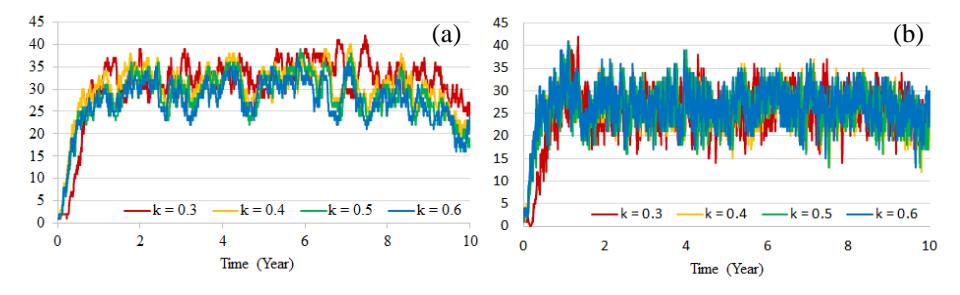
Figure 2 Dynamics of infected human population (a) and infected mosquito population (b) for Scenario 1.
Fig. 3 shows that the higher the value of , the more time is required to reach a disease-free equilibrium for a set given initial values (ℎ (0), (0)). Moreover, this time increases dramatically if the vector's initial value increases from (ℎ (0), (0)) = (0,1) to (ℎ (0), (0)) = (0,10). If the initial values for humans increase (ℎ (0), (0)) = {(1,0), (2,0), (3,0)}, then the time required to reach a disease-free equilibrium is slightly shorter. After experiencing a downturn, it gradually rises and remains steady at 6.22 × 10¹¹ years for = 0.3; remains steady at 3.13 × 10¹² years for = 0.4; remains steady at 7.89 × 10¹² years for = 0.5; and remains steady at 1.00 × 10¹³ years for = 0.6.
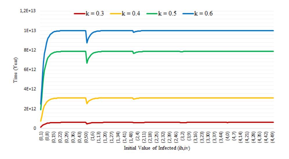
Figure 3 Expected time to reach a disease-free equilibrium for Scenario 1.
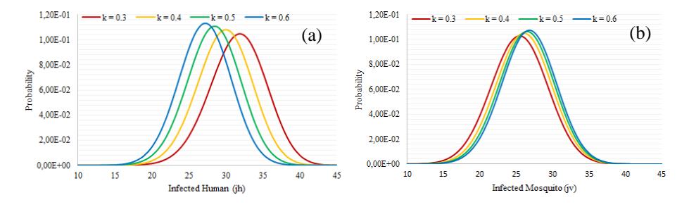
Figure 4 Quasi-stationary probability distribution of infected human (a) and infected mosquito (b) for Scenario 1.
Based on Fig. 4 it can be seen that for a curve with legend = 0.3, the highest probability occurs when ℎ = 32 and = 25. This means that before a diseasefree equilibrium is reached, 32 infected humans and 25 infected mosquitoes will be found in the system. This is the same for = 0.4, when the greatest probability occurs for ℎ = 30 and = 26; for = 0.5, when the greatest probability occurs for ℎ = 28 and = 26; and for = 0.6, when the greatest probability occurs for ℎ = 27 and = 27.
The quasi-stationary distribution shown in Fig. 4 indicates that the expected numbers of infected humans for = 0.3, = 0.4, = 0.5, and = 0.6 are 31.6, 29.8, 28.4, and 27.1, respectively. Meanwhile, the expected numbers of infected mosquitoes for = 0.3, = 0.4, = 0.5, and = 0.6 are 25.4, 26.0, 26.4, and 26.7, respectively. In this scenario, we obtain that the value of may affect the number of infected humans and infected mosquitoes before the disease-free equilibrium is reached. Thus, we can conclude that the value of increases with the number of infected mosquitoes but decreases with the number of infected humans.
4.2 Scenario 2: The Effect of Changing the Effectiveness of the Human Immunity System ()
In this scenario, the value of parameter , the effectiveness of the human immunity system, was varied. The parameter values used, = 0.5 and = 0.5, were assigned to be constant. The simulation results are presented in terms of the obtained value of ℛ0, the probability of disease outbreak, and the expected time required to reach a disease-free equilibrium (See Table 3).
The results in Table 3 show that an increase of will decrease ℛ0, the outbreak probability and also the expected time required until a disease-free equilibrium is reached.
| Table 3 | Values of ℛ0 | , outbreak probability, and expected time required to | ||||
|---|---|---|---|---|---|---|
| reach a disease-free equilibrium. |
| 𝜽 | 𝓡𝟎 | Outbreak Probability | Expected Time (Years) |
|---|---|---|---|
| 0 | 8.04988 | 0.87324 | 1.72 × 10¹³ |
| 0.5 | 4.02494 | 0.74648 | 3.33 × 10⁷ |
| 0.7 | 2.41496 | 0.57746 | 648.186 |
| 0.9 | 0.80499 | 0 | 0.98882 |
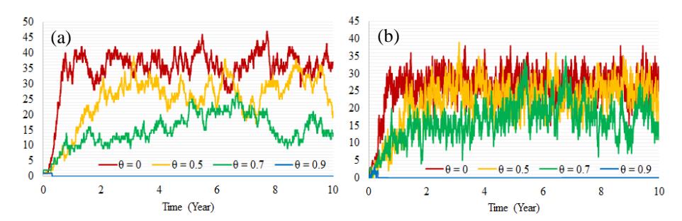
Figure 5 Dynamics of infected human population (a) and infected mosquito population (b) for Scenario 2.
Fig. 5 shows that the dynamics of infected humans and vectors ℎ and for = 0 and = 0.5 have relatively similar fluctuating patterns. This is maintained for a considerable period of time (see Table 3). Further, for = 0.7 the same fluctuating pattern occurs but in a slightly lower range. For = 0.9 the pattern is maintained with an even lower range of infected humans and mosquitoes. For this latter value, the disease-free equilibrium is reached within less than one simulation year.
Fig. 6 shows that the higher the value of , the shorter the time required to reach a disease-free equilibrium for a set of initial values (ℎ(0),(0)). However, this time increases dramatically if the vector's initial value increases from (ℎ(0),(0)) = (0,1) to (ℎ(0),(0)) = (0,10). For several initial values, except (0) = 0, the time required to reach a disease-free equilibrium dropped slightly but gradually rises and remains steady at 1.97 × 10¹³ years for = 0; steady at 4.52 × 10⁷ years for = 0.5; steady at 1182.56 years for = 0.7; and steady 4.04 years for = 0.9.
From Fig. 7 it can be seen that for the = 0 curve, the highest probability occurs when ℎ = 37 and = 27. This means that before the disease-free equilibrium is reached, often 37 infected humans and 27 infected mosquitoes will be found in the system. This is the same for = 0.5, where the greatest probability occurs when ℎ = 27 and = 23; for = 0.7 it occurs when ℎ = 17 and = 18; and for = 0.9 it occurs when ℎ = 0 and = 1.
The quasi-stationary distribution shown in Fig. 7 indicates that the expected value of the numbers of infected humans for = 0, = 0.5, = 0.7, and = 0.9 are 36.2, 26.3, 16.6, and 0.97, respectively. Meanwhile, the expected value of the number of infected mosquitoes for = 0, = 0.5, = 0.7, and = 0.9 are 27.1, 23.0, 17.3 and 1.96, respectively. In this scenario, we obtain that the value of may affect the number of infected humans and infected mosquitoes
before the disease-free equilibrium is reached. Thus, we can conclude that an increase of decreases the number of infected humans before the disease-free equilibrium is reached.
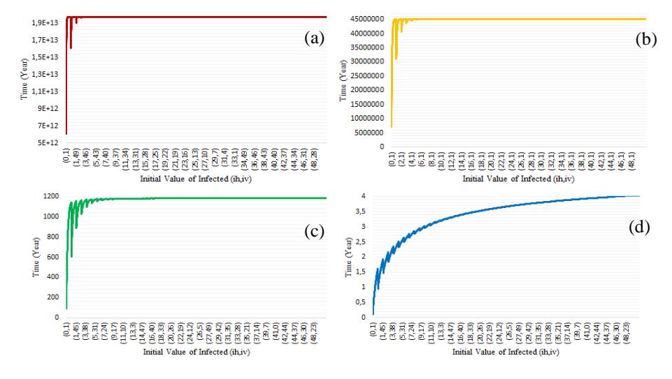
Figure 6 Expected time to reach a disease-free equilibrium with = 0 (a), = 0,5 (b), = 0,7 (c), and = 0,9 (d) for Scenario 2.
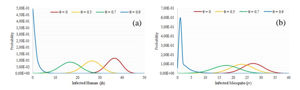
Figure 7 Quasi-stationary probability distribution of infected human (a) and infected mosquito (b) for Scenario 2.
5 Conclusions
From this work it is concluded that if the probability that a mosquito bites an infectious human () increases malaria disease will spread quickly. Thus, the outbreak probability will be higher and the expected time required to reach a disease-free equilibrium will be much longer. On the other hand, an increase of effectiveness of the human immunity system () will slow down the spread of the malaria disease. Also, it may be concluded that both the outbreak probability and the expected time required to achieve a disease-free equilibrium will be shorter.
The computer simulation denoted as Scenario 2 is aligned with the modified Chamchod and Britton's model, considering an immunity factor of = 0.3. As a result, the probability of disease outbreak decreases from 0.87324 to 0.74648. Similarly, the expected time to reach a disease-free equilibrium is much shorter, decreasing from 1.72 × 10¹³ to 3.33 × 10⁷ simulation years.
The quasi-stationary probability can describe the number of infected individuals in the population before a disease-free equilibrium is reached with a certain probability value. Based on the simulation results it was found that and may affect the number of infected humans and mosquitoes before a disease-free equilibrium is reached. The value of increases with the number of infected mosquitoes, but it will decrease with the number of infected humans. On the other hand, an increase of may decrease both the number of infected humans and the number of infected mosquitoes before a disease-free equilibrium point is reached.