
1 Introduction
The world has been facing an epidemic of COVID-19, a new strain of coronavirus that first appeared in December 2019 in the capital of Hubei Province, China, where the virus rapidly spread among the residents. The general symptoms after getting COVID-2019 consist of fever, coughing, shortness of breath, weakness, fatigue, headache, and diarrhea [1]-[3]. Measures for alleviating the COVID-19 outbreak have been applied in all countries in the world. During the first wave of the COVID-19 outbreak, many countries imposed lockdowns to suppress the spread of the virus. However, these lockdowns have negatively affected the economy, especially, the industrial, service, and tourism sectors. After the first wave, the lockdowns were lifted in order to let the economy recover. Movement and migration of people were allowed again. This increased the risk of COVID-19 disease transmission among people [4][5]. Subsequently, a second wave of the COVID-19 outbreak emerged after relaxation of the preventive measures. This caused an increase in the number of COVID-19 cases from the first wave to the second wave. For example, according to the WHO Thailand Situation Report [6], Thailand had approximately 1,300 infected people during the first wave. During the second wave, the total number of cases was 15,465 people.
A model for predicting the number of infected people is an important tool to help governments develop policies to control severe epidemics. A lot of research has been done related to COVID-19 forecasting, using models such as the logistic growth model, the generalized logistic growth model, the Richards model, the simple Gaussian model, the Ratkowsky model, and compartment models for the first as well as for the second wave. Studying the logistic growth model, the generalized logistic growth model and the generalized Richards model for forecasting the number of infected cases in 29 provinces in China and other regions in the world, the findings revealed that different outbreak levels can be classified into three groups. The authors suggest that the forecasts in some countries are largely misleading due to several factors, such as case definition, testing capacity, testing protocols, and reporting system and time [7]. The logistic growth model, the generalized logistic growth model, and the generalized growth model were used for daily forecasting of confirmed cases in India [8]. The compartmental model (generalized SEIR model), the logistic growth model, and the simple Gaussian model for predicting the spread of COVID-19 were studied in Iraq and Egypt [9]. The Richards model, the Gompertz model, the logistic model, the Ratkowsky model, the compartmental model (SIRD model), and the SIR model were investigated for making projections of the COVID-19 pandemic dynamics in Iran [10][11]. The logistics model for estimating the number of COVID-19 cases in Sweden and other Nordic countries, the USA, Brazil, and India has been studied and validated for COVID-19 situation control policies, such as strict lockdown and herd immunity policies [12][13]. A comparison was made between utilizing the logistic growth model and the Gompertz growth model for estimating COVID-19 cumulative cases in Southeast Asian countries [14]. Meanwhile, a second wave has occurred in many countries in Europe, the United States, New York, and Asian countries [15]. The researchers compared an estimate of the second wave using the logistic model with the final size of the second wave. They found that the data followed the logistics curve during the first wave and then started to deviate from it, indicating the beginning of the second wave of the epidemic [16].
A question that challenges statisticians is how to identify when a second wave will occur and how long it will take to enter the so-called second wave phase and how long the delay time between the first and the second wave is, which is important to know when making decisions on policy-level planning to cope with severe pandemic outbreaks.
The present research focused on the delay time parameter and its confidence interval in relation to the first and the second wave of the COVID-19 outbreak based on the total number of COVID-19 cumulative cases in the four sampled countries of this research: Thailand, South Korea, Egypt, and Nigeria. By comparing the parameters of the logistic and the delay logistic growth model, their performance was measured in terms of the coefficient of determination and the root mean squared percentage error.
2 Materials and Methods
This section presents the mathematical and statistical background and the material and methods used in this research.
2.1 Data collection
The data used in this research were gathered from the Worldometers website [17]. This website provides data about the COVID-19 outbreak worldwide. The provided data consists of total coronavirus cases, daily new cases, active cases, total coronavirus deaths, daily new deaths, newly infected, newly recovered, recovery rate, and death rate, etc. However, the total numbers of coronavirus cases, i.e. the cumulative number of COVID-19 cases during the first and the second wave of the COVID-19 outbreak, were collected for this research. The sampled countries for this research were Thailand, South Korea, Egypt, and Nigeria. The period of collected data was from February 15, 2020 (t = 0) to January 10, 2021 (t = 330).
2.2 Predictive Time Series and Its Parameter Estimation for the COVID-19 Outbreak
The growth curve time series as a predictive time series for describing the COVID-19 outbreak is a solution to the logistic differential equations. The solution is called the logistic growth curve time series, which is a flattened curve after passing its inflection point. This property corresponds to the behavior of the COVID-19 outbreak [13][14]. Let T(t) be a logistic growth curve time series of the total COVID-19 cases at any time t. The logistic differential equation was developed in [18] as:
\[\frac{d}{dt}T(t) = rT(t) \left[ 1 - \frac{T(t)}{C} \right]; \ T(t=0) = T_0,\] (1)
where \(T_0\) is the initial condition for an infectious COVID-19 case, r is the intrinsic growth rate, t is the time, and C is the carrying capacity.
The Eq. (1) can be solved by a partial fraction and separable method [13][14]. Therefore, the logistic growth curve time series is carried out as follows:
\[T(t) = \frac{C}{(1 + K \exp(-rt))},\] where \(K = \frac{C - T_0}{T_0}\). (2)
Asymptotic behavior of the logistic growth curve time series will converge to the carrying capacity.
The inflection point of logistic growth curve time series is at \(\frac{C}{2}\), which is the maximum outbreak point, and it is equivalent to the peak time at \(t = \frac{\ln(C)}{r}\). The parameters K, r, C of the logistic growth curve time series can be estimated by the least square error method. Let e(t) be an error function of the difference between the actual and the estimated value at any time t. The sum square error S can be evaluated as follows:
\[S = \sum_{t=1}^{n} [e(t)]^{2} = \sum_{t=1}^{n} [actual(t) - estimate(t)]^{2}.\]
To minimize the sum square error, the partial derivative and setting to zero are computed by the calculus concept:
\[\frac{\partial S}{\partial K} = 0\] \[\frac{\partial S}{\partial r} = 0\] \[\frac{\partial S}{\partial c} = 0\] (3)
The optimal parameters or estimated parameters K, r, C can be solved by the least square error method. The validation and accuracy of the predictive growth curve time series are based on statistic the coefficient of determination (R<sup>2</sup>) and the root mean squared percentage error (RMSPE) [13][14].
2.3 Logistic Growth Curve Time Series of the Total COVID-19 Outbreak During the First and the Second Wave
The variables related to the analysis of the predictive time series of the first and the second wave of the COVID-19 outbreak are defined as shown in Figure 1. \(T_0\) denotes the initial total number of COVID-19 cases at starting time \(t_1\) of the first wave. \(C_1\) denotes the carrying capacity of the total number of COVID-19 cases at ending time \(t_{C1}\) of the first wave. Also, \(C_1\) will become the initial total number of COVID-19 cases at starting time \(t_2\) of the second wave. \(C_2\) denotes the carrying capacity of the total number of COVID-19 cases at ending time \(t_{C2}\) of the second wave. \(I_1\) denotes the inflection point of the first wave of the COVID-19 outbreak at time \(t_{I1}\), while \(I_2\) denotes the inflection point of the second wave of the COVID-19 outbreak at time \(t_{I2}\). Moreover, the delay time or lag time between the first and the second wave, denoted by \(\tau\), appears before the second wave. Based on the symmetric property of the logistic growth time series, the ending time of the first and the second wave can be evaluated as:
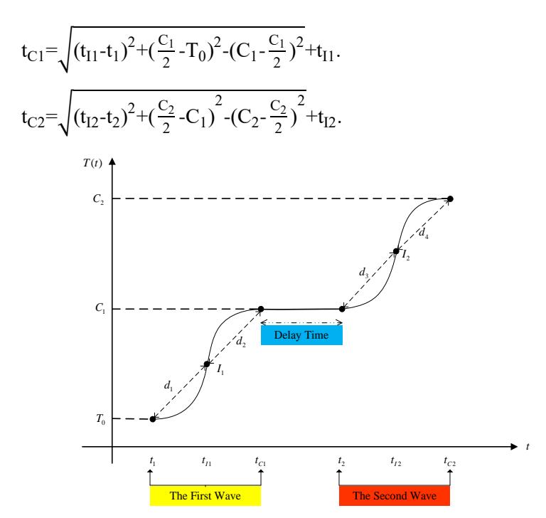
Figure 1 The structure of the predictive time series of the COVID-19 outbreak between the first and the second wave.
2.4 Analysis of Delay Time Between the First and the Second Wave of the COVID-19 Outbreak
2.4.1 Delay logistic growth time series for delay time between the first and the second wave
The delay logistic growth time series, a solution to the delay logistic differential equation, is more generalized than the logistic growth time series in Eq. (2). The logistic growth time series is under the assumption that the process relies on the growth rate of the relative number of individuals. On the other hand, the delay logistic growth time series is under the assumption that the time series process is not instantaneous. Thus, the delay logistic differential equation extended from the logistic differential equation in Eq. (4) can be defined as follows:
\[\frac{d}{dt}T(t) = rT(t-\tau)[1 - \frac{T(t)}{C}]; \quad T(t=0) = T_0,\] (4)
where \(\tau > 0\) is the delay time or lag time. An analytical solution of the delay logistic differential equation cannot be computed. A numerical solution, the method of steps, was adopted to solve this problem. The method of steps is conducted to transform the delayed logistic differential equations in a given interval to ordinary differential equations over that interval by using the iteration steps of the next interval [19]. Let \(T_0(t)\) be the initial condition function for the delay logistic differential equations. The process of the method of steps is given as:
- 1. 1<sup>st</sup> step: On the interval \(t \in [-\tau, 0]\), then \(T(t) = T_0(t)\).
- 2. \(2^{nd}\) step: On the interval \(t \in [0, \tau]\), then \(T(t-\tau) = T_0(t-\tau)\). The solution of the delay logistic differential equation \(\frac{d}{dt}T(t) = rT_0(t-\tau)[1-\frac{T(t)}{C}]\) as given \(T_1(t)\).
- 3. \(3^{rd}\) step: On the interval \(t \in [\tau, 2\tau]\), then \(T(t-\tau) = T_1(t-\tau)\). The solution of the delay logistic differential equation \(\frac{d}{dt}T(t)=rT_1(t-\tau)[1-\frac{T(t)}{C}]\) is solved as given \(T_1(t)\). The steps are continuously repeated until the desired time subsequent interval is reached.
2.4.2 Cross correlation for estimate delay time
The cross correlation [20] between two time series x(t) and y(t) can be given by:
\[Xcorr_{\tau}(x,y) = \int_{-\infty}^{\infty} x(t)y(t-\tau)dt\] for continuous time series \(x(t)\) and \(y(t)\)
\[X_{corr}(x,y) = \sum_{t=-\infty}^{\infty} x(t)y(t-\tau)\] for discrete time series \(x(t)\) and \(y(t)\), where \(\tau > 0\) is the delay time or lag time. This is useful for measuring the similarity between two time series and detecting the lag or delay of the two time series.
2.4.3 Confidence interval for delay time
In this research, the delay time between the first and the second wave of the COVID-19 outbreak was assumed to follow a uniform distribution on the interval \([t_{C1},t_2]\). Let t follow a uniform distribution on interval \([t_{C1},t_2]\) where \(t_{C1}\) is the minimum time and \(t_2\) is the maximum time. The probability density function (pdf) of the uniform distribution is defined as:
\[pdf: f(t;t_{C1},t_2) = \begin{cases} \frac{1}{t_2-t_{C1}}; \ t \in [t_{C1},t_2] \\ 0; \ t \notin [t_{C1},t_2] \end{cases}.\]
The cumulative distribution function (cdf) of the uniform distribution is defined as:
\[cdf: F(t; t_{C1}, t_2) = \begin{cases} 0; t < t_{C1} \\ \frac{t - t_{C1}}{t_2 - t_{C1}}; t \in [t_{C1}, t_2] \\ 1; t > t_2 \end{cases}\]
Let \(M_n\) be a statistic or an order statistics estimator \(Max(\{t_i \in [t_{C1},t_2]\})\) of independent and identically distributed random variables \(t_i \in [t_{C1},t_2]\). The cumulative distribution function of \(M_n\) can be derived as:
\[\mathbf{Pr}(\mathbf{M}_n \leq \mathbf{x}) = \mathbf{Pr}(\lceil \mathbf{T}_1 \leq \mathbf{x} \rceil \cap \lceil \mathbf{T}_2 \leq \mathbf{x} \rceil \cap ... \cap \lceil \mathbf{T}_n \leq \mathbf{x} \rceil) = \prod_{i=1}^n \mathbf{Pr}(\mathbf{T}_i \leq \mathbf{x}).\]
Thus, the cumulative distribution function of the maximum value \(M_n\) between \(t_{C1}\) and \(t_2\) is evaluated as:
\[cdf: F_{M_n}(t;t_{C1},t_2) = \prod_{i=1}^n F_{T_i}(t) = \begin{cases} 0; \ t < t_{C1} \\ \left(\frac{t - t_{C1}}{t_2 - t_{C1}}\right)^n; \ t \in [t_{C1},t_2] \\ 1; \ t > t_2 \end{cases}.\]
The probability density function of the maximum value \(M_n\) between \(t_{C1}\) and \(t_2\) is evaluated as:
\[pdf: f_{M_n}(t) = \frac{d}{dx} F_{T_n}(t) = \frac{n}{(t_2 - t_{C1})^n} (t - t_{C1})^{n-1} \text{ for } t_{C1} \le t \le t_2.\]
The expected value of \(M_n\) can be computed as:
\[\begin{split} \mathbf{E}(\mathbf{M}_n) &= \int_{t_{C1}}^{t_2} t f_{\mathbf{M}_n}(t) dt \\ &= \int_{t_{C1}}^{t_2} t \frac{n}{(t_2 - t_{C1})^n} (t - t_{C1})^{n-1} dt \\ &= \frac{n}{(t_2 - t_{C1})^n} \int_{t_{C1}}^{t_2} t (t - t_{C1})^{n-1} dt \\ &= \frac{n}{(t_2 - t_{C1})^n} \left[ \frac{(t_2 - t_{C1})^{n+1}}{n+1} + \frac{t_{C1}(t_2 - t_{C1})^n}{n} \right] \\ &= \frac{n(t_2 - t_{C1})}{n+1} + t_{C1}. \end{split}\]
The expected value of \((M_n)^2\) can be computed as:
\[\begin{split} E(M_n^2) &= \int_{t_{C1}}^{t_2} t^2 f_{M_n}(t) dt \\ &= \int_{t_{C1}}^{t_2} t^2 \frac{n}{(t_2 \cdot t_{C1})^n} (t \cdot t_{C1})^{n \cdot 1} dt \\ &= \frac{n}{(t_2 \cdot t_{C1})^n} \int_{t_{C1}}^{t_2} t^2 (t \cdot t_{C1})^{n \cdot 1} dt \\ &= \frac{n}{(t_2 \cdot t_{C1})^n} \bigg[ \frac{(t_2 \cdot t_{C1})^{n \cdot 2}}{n \cdot 2} + \frac{2t_{C1}(t_2 \cdot t_{C1})^{n \cdot 1}}{n \cdot 1} + \frac{(t_{C1})^2 (t_2 \cdot t_{C1})^n}{n} \bigg] \\ &= \frac{n(t_2 \cdot t_{C1})^2}{n \cdot 2} + \frac{2nt_{C1}}{n \cdot 1} (t_2 \cdot t_{C1}) + (t_{C1})^2. \end{split}\]
The variance of \(M_n\) can be computed as:
\[\begin{split} \textbf{Var}(\textbf{M}_n) &= \textbf{E}(\textbf{M}_n^2) - (\textbf{E}(\textbf{M}_n))^2. \\ &= \frac{\textbf{n}(t_2 - t_{C1})^2}{\textbf{n} + 2} + \frac{2\textbf{n}t_{C1}}{\textbf{n} + 1} \left(t_2 - t_{C1}\right) + (t_{C1})^2 - \left[\frac{\textbf{n}(t_2 - t_{C1})}{\textbf{n} + 1} + t_{C1}\right]^2. \end{split}\]
The estimator \(M_n\) can be transformed to an unbiased estimator by \(B_n = \frac{n+1}{n} M_n\), with the expected value and the variance are:
\[\mathbf{E}(\mathbf{B}_n) = \frac{n+1}{n} \mathbf{E}(\mathbf{M}_n)\]
\[\begin{split} &= \frac{n+1}{n} \left[ \frac{n(t_2 - t_{C1})}{n+1} + t_{C1} \right] \\ &\mathbf{Var}(B_n) = \left( \frac{n+1}{n} \right)^2 \mathbf{Var}(M_n) \\ &= \left( \frac{n+1}{n} \right)^2 \left\{ \frac{n(t_2 - t_{C1})^2}{n+2} + \frac{2nt_{C1}}{n+1} (t_2 - t_{C1}) + (t_{C1})^2 - \left[ \frac{n(t_2 - t_{C1})}{n+1} + t_{C1} \right]^2 \right\} \end{split}\]
To determine the confidence interval of the starting time t<sub>2</sub> of the second wave of the COVID-19 outbreak, Chebyshev's inequality is applied.
\(\text{Pr}(|B_n\text{-}t_2| \geq \epsilon) \leq \frac{\text{Var}(B_n)}{\epsilon^2} \text{ , where } \epsilon \text{ is any positive real number.}\)
\[\mathbf{Pr}(B_n + \varepsilon \ge t_2 \ge B_n - \varepsilon) \le \frac{\left(\frac{n+1}{n}\right)^2 \left\{\frac{n(t_2 - t_{C1})^2}{n+2} + \frac{2nt_{C1}}{n+1} (t_2 - t_{C1}) + (t_{C1})^2 - \left[\frac{n(t_2 - t_{C1})}{n+1} + t_{C1}\right]^2\right\}}{\varepsilon^2}\]
\[\text{[rumus tidak dapat ditampilkan dengan baik — lihat PDF asli]}\]
\[\text{where } \epsilon = \sqrt{\frac{\left(\frac{n+1}{n}\right)^2 \left\{\frac{n(t_2 - t_{C1})^2}{n+2} + \frac{2nt_{C1}}{n+1}(t_2 - t_{C1}) + (t_{C1})^2 - \left[\frac{n(t_2 - t_{C1})}{n+1} + t_{C1}\right]^2\right\}}{\alpha}}.\]
Then, the confidence interval \((1-\alpha)100\%\) for starting time \(t_2\) of the second wave of the COVID-19 outbreak is \(B_n\)-\(\epsilon\) for the lower confidence limit (LCL) and \(B_n\)+\(\epsilon\) for the upper confidence limit (UCL). Therefore, the confidence interval \((1-\alpha)100\%\) for the delay time between the first and the second wave of the COVID-19 outbreak is \(t_{C1}\)-\(\epsilon\) for LCL and \(\frac{n+1}{n}B_n\)+\(\epsilon\) for the UCL.
3 Results and Discussion
In this section, the results of this research are demonstrated and interpreted.
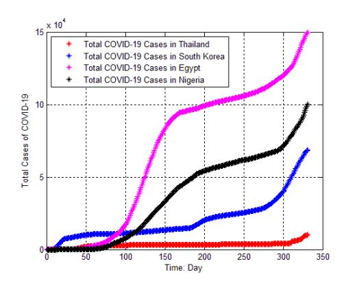
Figure 2 The total numbers of COVID cases for the four sampled countries.
The total numbers of COVID-19 cases for the four countries are shown in Figure 2. Thailand had a relatively low and the flattest infection trend, followed by South Korea, Nigeria, and Egypt, respectively. According to Figure 2, the total number of COVID-19 cases in the four countries from starting point to around day 150 was flat. Then, the rate of increase in the cumulative infections was relatively steady or became slightly higher from day 151 to day 300. Especially the total number of COVID-19 cases in Egypt was quite high compared with the other countries.
3.1.1 Comparison and Analysis of Predictive Time Series on COVID-19 Outbreak Between the First and the Second Wave in Thailand
The logistic and delay logistic time series for the estimated total number of COVID-19 cases during the first wave in Thailand are shown in Figure 3(a) and 3(b), respectively. The real total number of COVID-19 cases is indicated by the circle, while the solid line indicates the estimated total number of COVID-19 cases. It can be seen that the number of infections estimated by the logistic time series was a better match than that of the delay logistic time series for the first wave of the COVID-19 outbreak. The cross correlations showed that the estimated delay time for the second wave was approximately 90 days after the first wave, as can be seen in Figure 4(a). Namely, from day 0 to 330, the first date of the second wave was day 91. The prediction of the time series of the total number of COVID-19 cases during the second wave showed that the delay logistic time series is preferable. It showed that the logistic time series is not suitable for predicting the total number of COVID-19 cases, as shown in Figure 4(b).
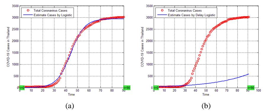
Figure 3 Logistic time series (a) and delay logistic time series (b) for the total number of COVID-19 cases during the first wave in Thailand.
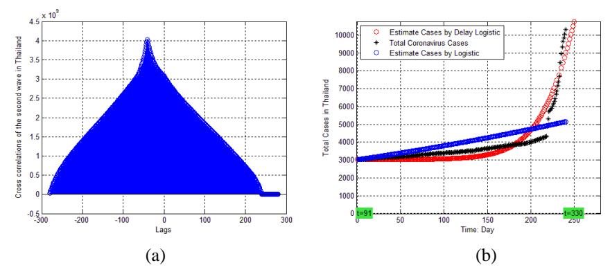
Figure 4 Cross correlations for estimated delay time (a) and predictive time series for the total number of COVID-19 cases (b) during the second wave in Thailand.
3.1.2 Comparison and Analysis of Predictive Time Series on COVID-19 Outbreak Between the First and the Second Wave in South Korea
The logistic and delay logistic time series for the predicted total number of COVID-19 cases for the first wave in South Korea are shown in Figure 5(a). and 5(b), respectively. The real total number of COVID-19 cases is indicated by the circle while the solid line indicates the estimated total number of COVID-19 cases. It can be seen that the estimated total number of COVID-19 cases of the logistic time series was a better match than that of the delay logistic time series for the first wave. The cross correlations showed that the estimated delay time of the second wave was about 85 days after the first wave, as can be seen in Figure 6(a), from day 0 to 330, the first date of the second wave was day 86. The prediction of the time series of the total number of COVID-19 cases for the second wave showed that the logistic time series is preferable. It showed that the delay logistic time series was not suitable for explaining the total number of COVID-19 cases, as can be seen in Figure 6(b).
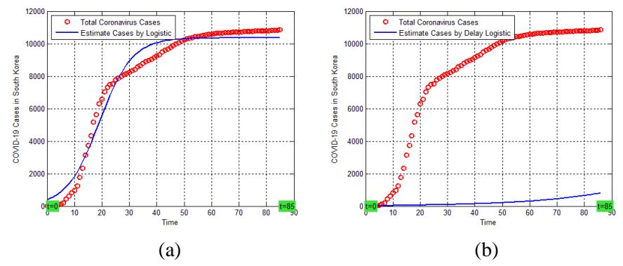
Figure 5 Logistic time series (a) and delay logistic time series for the total number of COVID-19 cases during the first wave in South Korea.
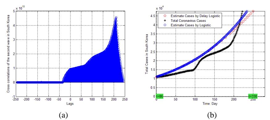
Figure 6 Cross correlations for estimated delay time (a) and predictive time series of the total number of COVID-19 cases (b) during the second wave in South Korea.
3.1.3 Comparison and Analysis of Predictive Time Series on COVID-19 Outbreak Between the First and the Second Wave in Egypt
The logistic and delay logistic time series for the predicted total number of COVID-19 cases during the first wave in Egypt are shown in Figure 7(a) and 7(b), respectively. The real total number of COVID-19 cases is indicated by the circle while the solid line indicates the estimated total COVID-19 cases. It was shown that the estimated total number of cases of infections from the logistic time series was a better match than that of the delay logistic time series for the first wave. The cross correlations showed that the estimated delay time for the second wave was about 220 days after the first wave, as can be seen in Figure 8(a). Namely, from day 0 to 330, the first date of the second wave was day 221. The prediction of the time series of the total number of COVID-19 cases for the second wave showed that the logistic time series and delay logistic time series performed equally well in this case, as shown in Figure 8(b).
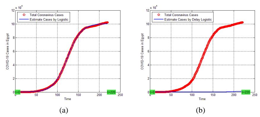
Figure 7 Logistic time series (a) and delay logistic time series (b) for the total number of COVID-19 cases during the first wave in Egypt.
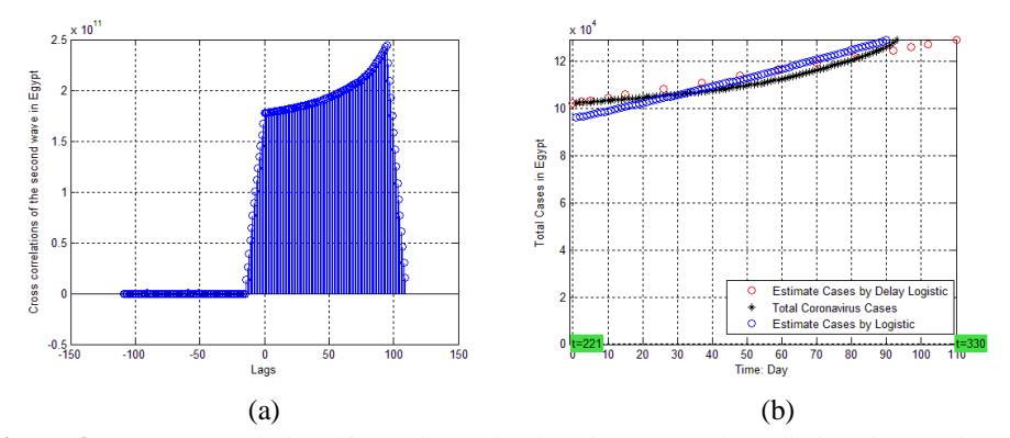
Figure 8 Cross correlations for estimated delay time (a) and predictive time series of the total number of COVID-19 cases (b) during the second wave in Egypt.
3.1.4 Comparison and Analysis of Predictive Time Series on COVID-19 Outbreak between the First and the Second Wave in Nigeria
The logistic and the delay logistic time series for the predicted total number of COVID-19 cases during the first wave in Nigeria are shown in Figure 9(a) and 9(b), respectively. The real total number of COVID-19 cases is indicated by the circle, while the solid line indicates the estimated total number of COVID-19 cases. It can be seen that the estimated total number of cases of infections by the logistic time series was a better match than that of the delay logistic time series for the first wave. The cross correlations showed that the estimated delay time for the second wave was about 210 days after the first wave, as shown in Figure 10(a). Namely, from day 0 to 330, the first date of the second wave was day 211. The prediction of the time series of the total number of COVID-19 cases for the second wave showed that the logistic time series and the delay logistic time series performed equally well, as can be seen in Figure 10(b).
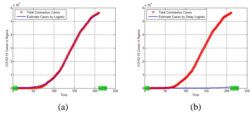
Figure 9 Logistic time series (a) and delay logistic time series (b) for the total number of COVID-19 cases during the first wave in Nigeria.
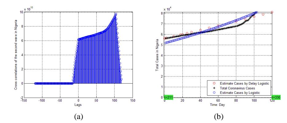
Figure 10 Cross correlations for estimated delay time (a) and predictive time series of the total number of COVID-19 cases (b) during the second wave in Nigeria.
3.1.5 Discussion and Comparison
A comparison of the parameter estimations of the logistic and the delay logistic time series for the first wave and the second wave of the COVID-19 outbreak is provided in Tables 1 and 2, respectively. The accuracy of the predictive time series of the total number of COVID-19 cases from the logistic and delay
logistic time series is based on the maximum of the coefficient of determination, which should approach one, and the minimum of the root mean squared percentage error, which should approach zero.
Table 1 Parameter Estimation of Logistic and Delay Logistic Time Series for COVID-19 Outbreak During the First Wave
| Country | T0 | Logistic Time Series | Delay Logistic Time Series | |||||
|---|---|---|---|---|---|---|---|---|
| r | C | R2 RMSPE | r | C | τ | R2 RMSPE | ||
| Thailand | 34 | 0.167 | 2946 | 0.998* 0.206* | 0.191 | 3025 | 14 | 0.862 0.634 |
| South Korea | 28 | 0.167 | 10358 | 0.977* 0.668* | 0.185 | 10874 | 8 | 0.512 240 |
| Egypt | 1 | 0.061 | 100385 | 1.000* 0.968* | 0.044 | 102254 | 6 | 0.456 560 |
| Nigeria | 1 | 0.043 | 58314 | 0.999* 0.988* | 0.0539 | 112354 | 12 | 0.857 615 |
Note: *appropriate value
Table 1 shows the estimated parameters of the logistic and the delay logistic time series for the the first wave of the COVID-19 outbreak. The validation and accuracy of the logistic time series for the first wave were based on \(R^2\) and RMSPE: Thailand (0.998, 0.206), South Korea (0.977, 0.668), Egypt (1.000, 0.968), and Nigeria (0.999, 0.988). Meanwhile, the validation and accuracy of the delay logistic time series for the first wave were Thailand (0.862, 0.634), South Korea (0.512, 240), Egypt (0.456, 560), and Nigeria (0.857, 615).
Table 2 shows the estimated parameters of the logistic and the delay logistic time series for the second wave of the COVID-19 outbreak. The validation and accuracy of the logistic time series for the second wave were based on R<sup>2</sup> and RMSPE: Thailand (0.473, 0.027), South Korea (0.895, 1.992), Egypt (0.883, 0.019), and Nigeria (0.863, 0.042). Meanwhile, the validation and accuracy of the delay logistic time series for the second wave were: Thailand (0.874, 0.024), South Korea (0.984, 0.038), Egypt (0.983, 0.001), and Nigeria (0.973, 0.003).
Comparing Thailand, South Korea, Egypt, and Nigeria, the longest delay time for the first wave of the COVID-19 outbreak was in Thailand, i.e. 14 days. The longest delay time for the second wave of the COVID-19 outbreak was in South Korea, i.e. 198 days. Based on the accuracy and validation of the predictive time series among the four countries, the logistic time series provided an R<sup>2</sup> larger than and an RMSPE smaller than the delay logistic time series for the first wave. In contrast, the delay logistic time series provided an R<sup>2</sup> larger than and an RMSPE smaller than the logistic time series for the second wave. This implies that the logistic time series was more suitable for estimating the total
number for the first wave of the COVID-19 cases than the delay logistic time series; on the other hand, the delay logistic time series was more suitable for estimating the total number for the second wave of COVID-19 cases than the logistic time series.
Table 2 Parameter Estimation of Logistic and Delay Logistic Time Series for COVID-19 Outbreak During the Second Wave
| _ | Logis | tic Time S | Series | Delay Logistic Time Series | ||||
|---|---|---|---|---|---|---|---|---|
| Country | \(T_0\) | r | C | R2 RMSPE | r | C | \(\tau\) with \(\alpha = 0.05\) (LCL-UCL) | R2 RMSPE |
| Thailand | 3025 | 0.0028 | 20587 | 0.473 0.027 | 0.0045 | 20596 | 41 (86-140) | 0.874* 0.024* |
| South Korea | 10874 | 0.0063 | 2073313 | 0.895 1.992 | 0.0075 | 137328 | 198 (81-290) | 0.984* 0.038* |
| Egypt | 102254 | 0.0034 | 4518732 | 0.883 0.019 | 0.0035 | 299584 | 95 (216-323) | 0.983* 0.001* |
| Nigeria | 56256 | 0.0044 | 4746755 | 0.863 0.042 | 0.0048 | 200174 | 104 (206-322) | 0.973* 0.003* |
Note: *appropriate value
4 Conclusion
This research focused on the delay time parameters and estimating the confidence of the predictive time series, the logistic and the delay logistic time series for the first and the second wave of the COVID-19 outbreak using the total number of infections from four countries: Thailand, South Korea, Egypt, and Nigeria.
The findings showed that the logistic time series was more suitable for estimating the total number of COVID-19 cases for the first wave in these four countries and the delay logistic time series was more suitable for estimating the total number of COVID-19 cases for the second wave. The maximum delay time shows a slow outbreak; the minimum delay time shows a fast outbreak. For example, Thailand had the longest maximum delay time for the first wave, 14 days, compared to the other countries. This means that there was a relatively slow outbreak in Thailand. Thus, Thailand could effectively control the COVID-19 outbreak during the first wave. However, South Korea could effectively control the COVID-19 outbreak during the second wave, because a maximum delay time of 198 days occurred in South Korea. Egypt had a shorter minimum delay time for the first wave, 6 days, compared to Thailand, South Korea, and Nigeria. This shows that there was a fast outbreak in Egypt during the first wave. During the second wave, Thailand had a minimum delay time of 41 days. This shows that there was a fast outbreak in Thailand during the second wave. As discussed previously, the logistic time series was more appropriate to forecast the total number of COVID-19 cases for the first wave and the delay logistic time series was more appropriate for predicting the total number of COVID-19 cases during the second wave, but this is based on the numbers from only four countries: Thailand, South Korea, Egypt, and Nigeria. Future research could focus on the total number of COVID-19 cases from other countries in the world.