
1 Introduction
Africa is a black continent typically known as a hotbed of infectious diseases and xenophobic attacks. The latter phenomenon today is not only an African issue but a global problem. However, South Africa in the recent past has been the epicenter of xenophobic attacks worldwide [1]. Xenophobia is a psychological state of hostility (or inequality) or fear towards non-natives or foreigners (immigrants) in a particular country [2][3]. It is a social vice that is based on the politics of competitive exclusion [4].
Soyombo [5] discusses xenophobic conditions based on economic theory, where the poor and unemployed are the main drivers of xenophobia. This class of people is predominant in African countries. Interestingly, the lack of access to economic opportunities, education, and land in South Africa over the decades has been responsible for a high poverty index and the emergence of xenophobia in Africa. The first xenophobic epidemic was experienced near the late 19th
century. The 2019 xenophobic attack in South Africa started as a result of economic and political issues, because of which the xenophobes have a feeling (or fear) that foreigners are taking control of their economic livelihood [6].
Even though Wimmer [7] considers xenophobia as a tool used to reassure nationals of their safety in time of world crisis, the effects of xenophobia on individuals have brought about political and economic instability, extreme poverty and underdevelopment, bridged in bilateral agreements, war against nations and finally ending up in human deaths. Statistically speaking, the number of deaths related to xenophobia is estimated to have been 412 between May 2008 and June 2013 in Africa [1] and the recent xenophobic attacks, which started late August 2019, claimed at least 12 lives while thousands were displaced [8]. To change this ugly scenario generated by xenophobia in public space, bilateral agreements between inter-governments should be re-enforced as well as the current correctional measures such as the development of intervention programs to promote accountability and counter the culture of impurity and provision for election-monitoring mechanisms to ensure that officials are not elected on an anti-foreigner/anti-outsider platform, as outlined in [9][10].
Xenophobia has been a world problem that started centuries ago. The 2019 xenophobic attack on Nigerians and some other foreigners in South Africa have called for the need of mathematicians to examine the way this menace can be stopped in Africa. It seems the xenophobic epidemic has not received full attention in the mathematical world. Some social models provide mathematical modeling insights for future studies [11][12] and some mathematical models that explore the impacts of fear on the dynamics of prey-predator systems have been developed [13]-[16]. The present study sought to develop a predator-like model for the spread and control of xenophobia in Africa based on the predatorprey system with fear and group defense formulated by Sasmal & Takeuchi [16]. In this paper, we describe xenophobes as those indigenous people who participate in xenophobic attacks.
The rest of the paper is organized as follows. In Section 2 we present the materials and methods. General analysis of the formulated model is done in Section 3 and Section 4 presents the numerical results. The discussion and conclusion of the paper are given in Section 5.
2 Mathematical Formulation
The derivation of the xenophobic model is based on the principle of competitive exclusion of species or strains existing in an ecosystem. According to this principle [17], when n strains (or species) compete for the same resources in a
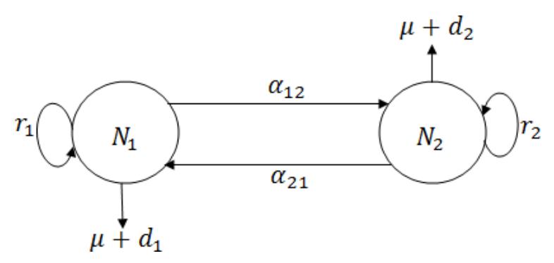
Figure 1 Competitive interactions between foreigners and xenophobes.
population, the strain with the largest reproduction number (super species) outcompetes the other strains and drives them to extinction.
Using the flow-diagram of the interacting population in Figure 1, we obtain the differential coefficient of the variables as indicated in Eq. (1)
The differential equation considering Figure 1 can be of the form
\[\begin{split} \frac{dN_1}{dt} &= Rate\ of\ change\ of\ N_1\ without\ N_2\ + \\ &\quad competitive\ effect\ of\ N_2\ on\ N_1, \\ \frac{dN_2}{dt} &= Rate\ of\ change\ of\ N_2\ without\ N_1\ + \\ &\quad competitive\ effect\ of\ N_1\ on\ N_2. \end{split}\]
The classical predator-prey system in Eq. (2) for competitive interaction by Sasmal & Takeuchi [16] was our guide for this formulation,
\[\frac{dx}{dt} = \frac{rx}{1+k\alpha y} - d_1 x - d_2 x^2 - \frac{\beta xy}{a+b\alpha x + x^2},\] \[\frac{dy}{dt} = c \frac{\beta xy}{a+b\alpha x + x^2} - my,\] (2)
where x is the prey density, and y is the density of predators. The description of the parameters in Eq. (2) can be found in Table 1 [16].
The following assumptions and the schematic diagram are useful for this study:
- 1. Indigenous people (xenophobes) and foreigners grow and compete logistically for the same resources.
- 2. Foreigners are considered to be prey to xenophobic attacks and xenophobes to be predators.
- 3. Xenophobes and foreigners may die naturally.
- 4. Foreigners decrease in the population as a result of xenophobic attacks.
- 5. The competitive effect of xenophobes on foreigners is greater than that of foreigners on xenophobes.
- 6. Holling type II incidence with anti-xenophobic behavior is introduced in the population of xenophobes.
Based on Eq. (1) with the application of Eq. (2), the mathematical model for xenophobic attacks can be given by
\[\frac{dN_1}{dt} = \frac{r_1 N_1}{1 + k(1 - \alpha)N_2} - \frac{r_1 N_1^2}{K_1} - \frac{r_1 \alpha_{12} N_1 N_2}{K_1 + b(1 - \alpha)N_1} - \mu N_1 - d_1 N_1,\] \[\frac{dN_2}{dt} = \frac{r_2 N_2}{1 + b(1 - \alpha)N_1} - \frac{r_2 N_2^2}{K_2} - \frac{r_2 \alpha_{21} N_2 N_1}{K_2 + m N_2} - \mu N_2 - d_2 N_2,\] (3)
where N1(0) > 0 and N2(0) > 0.
The variables and parameters of Eq. (3) are described in Tables (1) and (2) respectively.
Table 1 Variables of Eq. (3)
| Variables | Definition | |
|---|---|---|
| (𝑡) 𝑁1 | The population of foreigners in a particular country at time t | |
| (𝑡) 𝑁2 | The population of xenophobes in a particular country at time t | |
Table 2 Parameters of Eq. (3)
| Parameters | Definition | ||
|---|---|---|---|
| 𝑟1 , 𝑟2 | Economic growth rates of foreigners and xenophobes respectively | ||
| 𝐾1 ,𝐾2 | Specific carrying capacities of 𝑁1 and 𝑁2 respectively | ||
| 𝑑1 , 𝑑2 | Xenophobic induced death rates for 𝑁1 and 𝑁2 respectively | ||
| 𝛼12 | The competitive coefficient (attacking effect) on foreigners | ||
| 𝛼21 | The reverse competitive coefficient (retaliating effect) on xenophobes | ||
| 𝑚 | Anti-xenophobic behavior 𝑚 ∈ [0, 1] | ||
| 𝜇 | Natural death rate | ||
| 𝛼 | Rate of group defense against xenophobic attacks | ||
| 𝑘 | Level of fear possessed by foreigners | ||
| 𝑏 | Tolerance limit of xenophobes | ||
Note that = 1 implies that anti-xenophobic policy is not effective and = 0 means that the policy is effective with full implementation. We nondimensionalize Eq. (3) using the following equations:
\[\begin{aligned} x_1 &= \frac{N_1}{K_1}, x_2 = \frac{N_2}{K_2}, \beta_{12} = \alpha_{12} \frac{K_1}{K_2}, \ \beta_{12} = \alpha_{21} \frac{K_2}{K_1}, r = r_1 t, \rho = \frac{r_2}{r_1}, \\ \sigma_1 &= \frac{f_1}{r_1}, \sigma_2 = \frac{f_2}{r_2} \ with \ f_1 = \mu + d_1, f_2 = \mu + d_2, \ r_1, r_2 \in (0, 1). \end{aligned}\]
Thus, Eq. (3) becomes
\[\frac{dx_1}{dt} = \frac{x_1}{1 + k(1 - \alpha)K_2x_2} - x_1^2 - \frac{\beta_{12}x_1x_2}{1 + b(1 - \alpha)x_1} - \sigma_1x_1,\] \[\frac{dx_2}{dt} = \frac{\rho x_2}{1 + b(1 - \alpha)K_1x_1} - \rho x_2^2 - \rho \frac{\beta_{21}x_2x_1}{1 + mx_2} - \rho \sigma_2x_2,\] (4)
Any further analysis in this paper will be focused on the nondimensionalized Eq. (4). In the theorem below, we prove that the solutions of Eq. (4) are nonnegative and uniformly bounded.
Theorem 1 The set
\[\chi = \left\{ (x_1, x_2) \in R^2_+ \colon 0 \le \Gamma = x_1 + \ x_2 \le \frac{\xi}{\varphi} \right\}\] is an attractive domain for all solutions in the interior orthant, where is a positive constant such that
\[\xi = \frac{(R_1 + \varphi)^2}{4} + \frac{(\rho R_2 + \varphi)^2}{4\rho}.\]
Proof. The proof of Theorem 1 is guided by Sasmal & Takeuchi [16] and Lelu & Jiao [18]. Taking arbitrary 1, 2 > 0, we get
\[\left(\frac{dx_1}{dt}\right)|_{x_1=0} = \left(\frac{dx_2}{dt}\right)|_{x_2=0} = 0.\]
This shows that 1 = 0 and 2 = 0, are invariant manifolds respectively. Because of the fact that the solution of Eq. (4) is unique, we can deduce that the set 2 is periodically invariant. Let = 1() + 2() and > 0 be a constant. Then,
\[\frac{d\Gamma}{dt} = \frac{x_1}{1 + k(1 - \alpha)K_2x_2} + \frac{\rho x_2}{1 + b(1 - \alpha)K_1x_1} - x_1^2 - \frac{\beta_{12}x_1x_2}{1 + b(1 - \alpha)x_1} - \sigma_1 x_1 - \rho x_2^2 - \rho \frac{\beta_{21}x_2x_1}{1 + mx_2} - \rho \sigma_2 x_2.\]
Thus,
\[\begin{split} &\frac{d\Gamma}{dt} + \varphi\Gamma \leq (1 - \sigma_1 + \varphi)x_1 - x_1^2 + [\rho(1 - \sigma_2) + \varphi]x_2 - \rho x_2^2 \\ &= \frac{(R_1 + \varphi)^2}{4} - \left(x_1 - \frac{R_1 + \varphi}{2}\right)^2 + \frac{(\rho R_2 + \varphi)^2}{4\rho} - \rho \left(x_2 - \frac{\rho R_1 + \varphi}{2\rho}\right)^2 \leq \frac{(R_1 + \varphi)^2}{4\rho} + \frac{(\rho R_2 + \varphi)^2}{4\rho} \end{split}\]
\[=\xi\], where \(R_1 = 1 - \sigma_1\) and \(R_2 = 1 - \sigma_2\).
Applying the theorem on differential inequality, we get
\[0 \le \Gamma \big( x_1(t), x_2(t) \big) \le \frac{\xi}{\omega} \big( 1 - e^{-\xi t} \big) + \big( x_1(0), x_2(0) \big) e^{-\xi t}.\]
Taking the limit when \(t \to \infty\), we have
\[0 \le \Gamma(x_1(t), x_2(t)) \le \frac{\xi}{\varphi}\].
This completes the proof.
3 General Analysis of the Model
3.1 Existence of Equilibria
Here, it can be checked that the Eq. (4) has exactly four non-negative equilibria, namely, \(X_{00}(0,0), X_{10}(x_1,0), X_{02}(0,x_2)\), and \(X_{12}(x_1,x_2)\), denoting the trivial equilibrium, xenophobic-free equilibrium, xenophobic survival equilibrium, and the coexistence equilibrium respectively. The equilibrium point \(X_{00}(0,0)\) exists trivially, and we can prove the existence of \(X_{10}(x_1,0), X_{02}(0,x_2)\), and \(X_{12}(x_1,x_2)\) as follows:
3.2 Existence of \(X_{10}(x_1, 0), X_{02}(0, x_2), \text{ and } X_{12}(x_1, x_2)\)
Let \(x_1\), \(x_2\) be the non-negative solutions of the equations
\[0 = \frac{x_1}{1 + k(1 - \alpha)K_2 x_2} - x_1^2 - \frac{\beta_{12} x_1 x_2}{1 + b(1 - \alpha)x_1} - \sigma_1 x_1, \tag{5}\]
\[0 = \frac{\rho x_2}{1 + b(1 - \alpha)K_1 x_1} - \rho x_2^2 - \rho \frac{\beta_{21} x_2 x_1}{1 + m x_2} - \rho \sigma_2 x_2, \tag{6}\] when \(x_2 = 0\) and \(x_1 \neq 0\) then Eq. (5) reduces to
\[1-x_1-\sigma_1=0.\]
Thus,
\[X_{10} = (\underline{x}_1, 0) = (R_1, 0), where R_1 = 1 - \sigma_1.\]
Similarly, when xenophobes drive foreigners away completely from their country \((x_1 = 0)\), then Eq. (6) becomes
\[1-x_2-\sigma_2=0.\]
Hence,
\[X_{02} = (0, \underline{x}_2) = (0, R_2)\], where \(R_2 = 1 - \sigma_2\).
Furthermore, for the coexistence equilibrium 12 = (1, 2) when 1, 2 > 0 and 1, 2 are solutions of the following equations
\[0 = \frac{1}{1 + k(1 - \alpha)K_2 x_2} - x_1 - \frac{\beta_{12} x_2}{1 + b(1 - \alpha)x_1} - \sigma_1,\tag{7}\]
\[0 = \frac{1}{1 + b(1 - \alpha)K_1 x_1} - x_2 - \frac{\beta_{21} x_1}{1 + m x_2} - \sigma_2,\] (8)
For a specific case when = 1 and = 0, 12 is given as
\[X_{12} = \begin{pmatrix} \frac{R_1 - R_2 \beta_{12}}{1 - \beta_{12} \beta_{21}}, \frac{R_2 - R_1 \beta_{21}}{1 - \beta_{12} \beta_{21}} \end{pmatrix}\] which is shown by the phase portrait in Figure 2(a). Whereas for the general solution when ≠ 1 and ≠ 0, we have 12 = (1, 2), as displayed numerically in Figure 2(b).
3.3 Local Stability Analysis
To examine the local stability analysis of the equilibrium points, we compute the community matrix around each equilibrium state of Eq. (4). The community matrix of the model at any arbitrary state is:
\[J = \begin{pmatrix} l_{11} & -l_{12} \\ -l_{21} & l_{22} \end{pmatrix}, \tag{9}\] with
\[\begin{split} l_{11} &= \frac{1}{1 + k(1 - \alpha)K_2 x_2} - 2x_1 - \sigma_1 - \frac{\beta_{12} x_2}{(1 + b(1 - \alpha)x_1)^2}, \\ l_{12} &= x_1 \left( \frac{k(1 - \alpha)K_2}{(1 + k(1 - \alpha)K_2 x_2)^2} + \frac{\beta_{12}}{1 + b(1 - \alpha)x_1} \right), \\ l_{21} &= \rho x_2 \left( \frac{b(1 - \alpha)K_1}{(1 + b(1 - \alpha)K_1 x_1)^2} + \frac{\beta_{21}}{1 + m x_2} \right), \end{split}\] and
\[l_{22} = \frac{\rho}{1 + b(1 - \alpha)K_1x_1} - 2\rho x_2 - \rho \sigma_2 - \frac{\rho \beta_{21}x_1}{(1 + mx_2)^2}.\]
The underlined theorem proves the local stability analysis of equilibria.
Theorem 2
(a) The trivial equilibrium point 00 = (0,0) is unstable if 1 > 0 and 2 > 0
- (b) The xenophobic-free equilibrium point \(X_{10} = (\underline{x}_1, 0)\) is locally asymptotically stable if \(\frac{\rho}{1+b(1-\alpha)K_1R_1} < \beta_{21}R_1 + \sigma_2\)
- (c) The xenophobic survival equilibrium point \(X_{02} = (0, \underline{x}_2)\) is locally asymptotically stable if \(\frac{\rho}{1+k(1-\alpha)K_2R_2} < \beta_{12}R_2 + \sigma_1\)
- (d) The coexistence equilibrium point \(X_{12} = (\underline{x}_1, \underline{x}_2)\) is locally asymptotically stable if \(\alpha = 1\) and m = 0.
Proof.
(a) The community matrix at \(X_{12} = (0,0)\) is given as
\[J(X_{00}) = \begin{pmatrix} R_1 & 0 \\ 0 & \rho R_2 \end{pmatrix}\] with eigenvalues \(\lambda_1 = R_1\), \(\lambda_2 = \rho R_2\), which is a saddle point (unstable), since \(R_1 > 0\), \(R_2 > 0\).
(b) In terms of the equilibrium point \(X_{10} = (\underline{x}_1, 0)\), the community matrix is
\[J(X_{10}) = \begin{pmatrix} -R_1 & -A_1 \\ 0 & A_2 \end{pmatrix},\] where \(A_1 = R_1 k (1 - \alpha) K_2 + \frac{\beta_{12} R_1}{1 + b(1 - \alpha) R_1}\), and \(A_2 = \rho \left( \frac{1}{1 + b(1 - \alpha) K_1 R_1} - \beta_{21} R_1 - \sigma_2 \right)\).
The eigenvalues of \(J(X_{10})\) are \(\lambda_1 = -R_1\) and \(\lambda_2 = A_2\). One can see that if \(A_2 > 0\), then \(X_{10}(\underline{x}_1, 0)\) is a saddle. If \(A_2 > 0 \Leftrightarrow \frac{1}{1+b(1-\alpha)K_1R_1} < \beta_{21}R_1 + \sigma_2\) is a stable node. If \(A_2 = 0\), i. e. \(\lambda_2 = 0\), we cannot draw a conclusion easily.
(c) Jacobian matrix of the model at \(X_{02} = (0, \underline{x}_2)\) is given by
\[J(X_{02}) = \begin{pmatrix} A_3 & 0 \\ -A_4 & -\rho R_2 \end{pmatrix},\] where \(A_3 = \frac{1}{1+b(1-\alpha)K_1R_2} - \beta_{12}R_2 - \sigma_1\), and \(A_4 = \rho R_2b(1-\alpha)K_1 + \frac{\rho\beta_{21}R_2}{1+mR_2}\).
with the eigenvalues \(\lambda_1 = A_3\) and \(\lambda_2 = -\rho R_2\). The Jacobian \(J(X_{02})\) has negative eigenvalues if \(A_3 < 0\). Thus, equilibrium point \(X_{02}\) is locally asymptotically stable if \(\frac{1}{1+b(1-\alpha)K_1R_2} < \beta_{12}R_2 + \sigma_1\). Otherwise, \(A_3 > 0\), we get a saddle and \(A_3 = 0\) gives rise to a situation where a conclusion cannot be drawn easily.
(d) This proof follows from the work of Dubey [19] by linearizing Eq. (4), taking into account the transformations
\[x_1 = x_1 + X, x_2 = x_2 + Y. (10)\]
Next, making use of the Liaponuv function, which is positive definite,
\[L(t) = \frac{X^2}{2} + \frac{Y^2}{2},\] and whose derivative is taken with respect to time along the linear version of model equations
\[L'(t) = XX' + YY', \tag{11}\]
having in mind that \(X' = x_1'\) and \(Y' = x_2'\). Evaluating Eq. (11) using Eq. (4) and its trajectories, we get
\[\text{[rumus tidak dapat ditampilkan dengan baik — lihat PDF asli]}\]
However, when \(\alpha = 1\) and m = 0, after simplification we have
\[L'(t) = -x_1(x_1 - \underline{x}_1)^2 - \rho x_2(x_2 - \underline{x}_2)^2 - (x_1 - \underline{x}_1)(x_2 - x_2)(\beta_{12}x_1 + \rho\beta_{21}x_2)\]
Using the transformation given in Eq. (10) yields
\[L'(t) = -(\underline{x}_1 + X)X^2 - \rho(\underline{x}_2 + Y)Y^2 - XY(\beta_{12}(\underline{x}_1 + X) + \rho\beta_{21}(\underline{x}_2 + Y))\]
Undoubtedly, this shows that \(L(t) = \frac{X^2}{2} + \frac{Y^2}{2}\) is a Lyapunov function since L'(t) < 0. Thus, the proof is completed.
Table 3 summarizes the existence and local stability criteria of equilibria for Eq. (4).
| Equilibrium | Existence Criteria | Stability Criteria |
|---|---|---|
| \(X_{00} = (0.0)\) | Exist | \[R_1 < 0, R_2 < 0\] |
| \[X_{10} = (R_1, 0)\] | \(R_1 > 0\) | \[\frac{1}{1 + b(1 - \alpha)K_1R_1} < \beta_{21}R_1 + \sigma_2\] |
| \[X_{02} = (0, R_2)\] | \(R_2 > 0\) | \[\frac{1}{1 + b(1 - \alpha)K_1R_2} < \beta_{12}R_2 + \sigma_1\] |
| \[X_{12} = \frac{\binom{R_1 - R_2 \beta_{12}}{1 - \beta_{12} \beta_{21}}, \frac{R_2 - R_1 \beta_{21}}{1 - \beta_{12} \beta_{21}}}{\binom{R_2 - R_1 \beta_{21}}{1 - \beta_{12} \beta_{21}}}\] | \[R_2 \beta_{12} < R_1 < \frac{R_2}{\beta_{21}},\]\[\beta_{12} \beta_{21} < 1\] | \(\alpha = 1, m = 0\) |
Table 3 Existence and Local Stability Criteria for Eq. (4)
3.4 Global Analysis
The global behavior of the non-dimensionalized equations can be looked into by establishing the following theorems:
Theorem 3. Eq. (4) under the conditions \(\alpha = 1\) and m = 0 cannot exhibit any periodic solution in the interior of the positive quadrant of the \(x_1, x_2\) plane.
Proof. Let \(D(x_1, x_2) = \frac{1}{x_1 x_2}\) be a positive Dulacs function. Clearly, \(D(x_1, x_2)\) is positive in the interior of the positive quadrant of the \(x_1, x_2\) plane. Let
\[g_1(x_1, x_2) = \frac{x_1}{1 + k(1 - \alpha)K_2x_2} - x_1^2 - \frac{\beta_{12}x_1x_2}{1 + b(1 - \alpha)x_1} - \sigma_1x_1,\] \[g_2(x_1, x_2) = \frac{\rho x_2}{1 + b(1 - \alpha)K_1x_1} - \rho x_2^2 - \rho \frac{\beta_{21}x_2x_1}{1 + mx_2} - \rho \sigma_2x_2.\]
Then,
\[\nabla \left( g(x_1, x_2) D(x_1, x_2) \right) = \frac{\partial}{\partial x_1} (Dg_1) + \frac{\partial}{\partial x_2} (Dg_2)\] \[= -\frac{\rho}{x_1} - \frac{1}{x_2} + \left( \frac{\beta_{12} b(1 - \alpha)}{(1 + b(1 - \alpha)K_1 x_1)^2} \right) + \left( \frac{\rho \beta_{21} m}{(1 + m x_2)^2} \right) < 0,\] if \(\alpha = 1, m = 0\).
From the above relation, we notice that \(\nabla(x_1, x_2)\) does not deviate in sign and is not identical to zero in the interior of the positive first quadrant of the \(x_1, x_2\) plane. Therefore, it follows by the Bendixon-Dulac criteria [20] that there is no closed orbit, which implies that the system has no limit cycle in the interior of \(X_{12}\) and that ends the proof.
Theorem 4. The coexistence equilibrium point \(X_{12}\) for Eq. (4) is globally asymptotically stable with respect to all solutions in the interior of the positive order when \(\alpha = 1\) and m = 0.
Proof. Consider the following positive definite function about \(X_{12}\)
\[L_{12}(t) = c_1 \left( x_1 - \underline{x}_1 - \underline{x}_1 \ln \frac{x_1}{x_1} \right) + c_2 \left( x_2 - \underline{x}_2 - \underline{x}_2 \ln \frac{x_2}{x_2} \right)\] as applied in Dubey [19] with \(c_1\) and \(c_2\) being positive constants to be determined. The derivative of \(L_{12}(t)\) with respect to time along Eq. (4) gives
\[L'_{12}(t) = \left(1 - \frac{x_1}{x_1}\right) c_1 \left(\frac{x_1}{1 + k(1 - \alpha)K_2 x_2} - x_1^2 - \frac{\beta_{12} x_1 x_2}{1 + b(1 - \alpha)x_1} - \sigma_1 x_1\right) + \left(1 - \frac{x_2}{x_2}\right) c_2 \left(\frac{\rho x_2}{1 + b(1 - \alpha)K_2 x_2} - \rho x_2^2 - \rho \frac{\beta_{21} x_2 x_1}{1 + m x_2} - \rho \sigma_2 x_2\right).\]
But at equilibrium state
\[\sigma_{1} = \frac{1}{1 + k(1 - \alpha)K_{2}\underline{x}_{2}} - \underline{x}_{1} - \frac{\beta_{12}\underline{x}_{2}}{1 + b(1 - \alpha)\underline{x}_{1}},\] \[\sigma_{2} = \frac{1}{1 + b(1 - \alpha)K_{1}\underline{x}_{1}} - \underline{x}_{2} - \frac{\beta_{21}\underline{x}_{1}}{1 + m\underline{x}_{2}}.\]
Making use of the solutions and simplifying gives
\[\begin{split} L'_{12}(t) &= -c_1 \Big(x_1 - \underline{x_1}\Big)^2 - c_2 \Big(x_2 - \underline{x_2}\Big)^2 - c_1 \Big(x_1 - \underline{x_1}\Big) \Big(x_2 - \underline{x_2}\Big)^2 \\ &= \underline{x_2}\Big) \Big(\frac{k(1-\alpha)K_2}{(1+k(1-\alpha)K_2x_2) \Big(1+k(1-\alpha)K_2\underline{x_2}\Big)} + \\ &= \frac{\beta_{12}}{(1+b(1-\alpha)x_1) \Big(1+b(1-\alpha)\underline{x_1}\Big)} \Big) + \frac{c_2\beta_{21}m\underline{x_1} \Big(x_2 - \underline{x_2}\Big)^2}{(1+mx_2) \Big(1+m\underline{x_2}\Big)} - c_2 \Big(x_2 - \underline{x_2}\Big) \Big(x_1 - \underline{x_1}\Big) \Big(\frac{b(1-\alpha)K_1}{(1+b(1-\alpha)K_1x_1) \Big(1+b(1-\alpha)K_1\underline{x_1}\Big)} + \\ &= \frac{\beta_{21}m}{(1+mx_2) \Big(1+mx_2\Big)} \Big) + \frac{c_1\beta_{12}b(1-\alpha)\underline{x_2} \Big(x_1 - \underline{x_1}\Big)^2}{(1+b(1-\alpha)x_1) \Big(1+b(1-\alpha)x_1\Big)}. \end{split}\]
Setting \(\alpha = 1\) and m = 0 gives
\[L'_{12}(t) = -c_1(x_1 - \underline{x}_1)^2 - c_2(x_2 - \underline{x}_2)^2 - (x_1 - \underline{x}_1)(x_2 - \underline{x}_2)(c_1\beta_{12} + c_2\beta_{21}).\]
Thus, for any \(c_1, c_2 > 0\), \(L'_{12}(t) \le 0\) if \(\underline{x}_1 \le x_1\) and \(\underline{x}_2 \le x_2\) that is negative definite. Therefore, \(L_{12}(t)\) is a Lyaponuv function in \(X_{12}\) whose region contains the domain of attraction \(R_+^2\) and this completes the proof.
3.5 Local Bifurcation Analysis
In this subsection we discuss variable bifurcations of Eq. (4) and achieve conditions for transcritical bifurcation and saddle-node bifurcation. The proof of the following theorems explains it better.
Theorem 5. Eq. (4) has:
- 1. Transcritical bifurcation
- 2. No saddle-node bifurcation
- (a) near the xenophobic-free equilibrium point \(X_{10} = (\underline{x}_1, 0)\) when \(\sigma_1 = \sigma_1^* = 1\) and \(\sigma_2 < 1\);
- (b) near xenophobic survival equilibrium point \(X_{02} = (0, \underline{x}_2)\) when \(\sigma_2 = \sigma_2^* = 1\) and \(\sigma_1 < 1\), where \(\sigma_1, \sigma_2\) are the bifurcation parameters in (a) and (b) respectively;
- (c) near the positive coexistence equilibrium point \(X_{12} = (\underline{x}_1, \underline{x}_2)\) when the system parameters satisfy the restriction \(\beta_{12} = \beta_{12}^* = \frac{R_1}{R_2}\). Here, \(\beta_{12}\) is seen as the bifurcation parameter.
Proof
(a) Here, we use Sotomayor's theorem [21] to prove the existence of a transcitical bifurcation with the transversality condition. The Jacobian matrix about equilibrium \(X_{10}\) is given by
\[J(X_{10}) = \begin{pmatrix} 0 & 0 \\ 0 & \rho R_2 \end{pmatrix} = J(X_{10})^T.\]
Evidently, \(J(X_{10})\) has a zero-eigenvalue denoted by \(\lambda_1\). Let U and W be two eigenvectors respectively corresponding to the eigenvalue \(\lambda_1\) for the matrices \(J(X_{10})\) and \(J(X_{10})^T\). After simple calculation, we have
\[U = \begin{pmatrix} u_1 \\ u_2 \end{pmatrix} = \begin{pmatrix} 1 \\ 0 \end{pmatrix}, W = \begin{pmatrix} w_1 \\ w_2 \end{pmatrix} = \begin{pmatrix} 1 \\ 0 \end{pmatrix}.\]
Besides that,
\[\begin{split} F_{\sigma_1}(X_{10};\sigma_1^*) &= \binom{-x_1}{0}_{(x_1 = \bar{x}_1)} = \binom{0}{0}, \\ DF_{\sigma_1}(X_{10};\sigma_1^*)U &= \binom{-1}{0}_{0} \binom{0}{0}_{(X_{10};\sigma_1^*)} \times \binom{1}{0} = \binom{-1}{0}, \\ D^2F(X_{10};\sigma_1^*)(U,U) &= \binom{u_1^2 \frac{\partial^2 f_1}{\partial x_1^2} + 2u_1u_2 \frac{\partial^2 f_1}{\partial x_1\partial x_2} + u_2^2 \frac{\partial^2 f_1}{\partial x_2^2}}{u_1^2 \frac{\partial^2 f_2}{\partial x_1^2} + 2u_1u_2 \frac{\partial^2 f_2}{\partial x_1\partial x_2} + u_2^2 \frac{\partial^2 f_2}{\partial x_2^2}} \right)_{(X_{10};\sigma_1^*)} \\ &= \binom{-2}{0}. \end{split}\]
One can see that U and W satisfy
\[\begin{split} W^T F_{\sigma_1}(X_{10}; \sigma_1^*) &= 0, \\ W^T \big[ D F_{\sigma_1}(X_{10}; \sigma_1^*) U \big] &= -1 \neq 0, \\ W^T \big[ D^2 F(X_{10}; \sigma_1^*) (U, U) \big] &= -2 \neq 0, \end{split}\] which means that when \(\sigma_1^* = 1\); \(\sigma_2 < 1\) transcritical bifurcation occurs at \(X_{10}\). This establishes the proof of Theorem 5(a).
(b) In a similar fashion, we use Sotomayor's theorem [21] to prove the existence of transcitical bifurcation with the transversality condition \(\sigma_2^* = 1\). The Jacobian matrix around equilibrium \(X_{02}\) of Eq. (4) with the restriction \(\sigma_2^* = 1\) is given by
\[J(X_{02}) = \begin{pmatrix} R_1 & 0 \\ 0 & 0 \end{pmatrix} = J(X_{02})^T.\]
Obviously, \(J(X_{02})\) has a zero-eigenvalue denoted by \(\lambda_1\). Let U and W be two eigenvectors respectively corresponding to the eigenvalue \(\lambda_2\) for the matrices \(J(X_{02})\) and \(J(X_{02})^T\). After a bit of algebra, we get
\[U = \begin{pmatrix} u_1 \\ u_2 \end{pmatrix} = \begin{pmatrix} 0 \\ 1 \end{pmatrix}, W = \begin{pmatrix} w_1 \\ w_2 \end{pmatrix} = \begin{pmatrix} 0 \\ 1 \end{pmatrix}.\]
Also,
\[\begin{split} F_{\sigma_{2}}(X_{02};\sigma_{2}^{*}) &= \begin{pmatrix} 0 \\ -\rho x_{2} \end{pmatrix}_{(x_{2} = \bar{x}_{2})} = \begin{pmatrix} 0 \\ 0 \end{pmatrix}, \\ DF_{\sigma_{2}}(X_{02};\sigma_{2}^{*})U &= \begin{pmatrix} 0 & 0 \\ 0 & -\rho \end{pmatrix}_{(X_{02};\sigma_{2}^{*})} \times \begin{pmatrix} 0 \\ 1 \end{pmatrix} = \begin{pmatrix} 0 \\ -\rho \end{pmatrix}, \\ D^{2}F(X_{02};\sigma_{2}^{*})(U,U) &= \begin{pmatrix} u_{1}^{2} \frac{\partial^{2} f_{1}}{\partial x_{1}^{2}} + 2u_{1}u_{2} \frac{\partial^{2} f_{1}}{\partial x_{1}\partial x_{2}} + u_{2}^{2} \frac{\partial^{2} f_{1}}{\partial x_{2}^{2}} \\ u_{1}^{2} \frac{\partial^{2} f_{2}}{\partial x_{1}^{2}} + 2u_{1}u_{2} \frac{\partial^{2} f_{2}}{\partial x_{1}\partial x_{2}} + u_{2}^{2} \frac{\partial^{2} f_{2}}{\partial x_{2}^{2}} \end{pmatrix}_{(X_{02};\sigma_{2}^{*})} \\ &= \begin{pmatrix} 0 \\ -2\rho \end{pmatrix}. \end{split}\]
Therefore, U and W satisfy
\[W^{T}F_{\sigma_{2}}(X_{02}; \sigma_{2}^{*}) = 0,\]
\(W^{T}[DF_{\sigma_{2}}(X_{02}; \sigma_{2}^{*})U] = -\rho \neq 0,\)
\(W^{T}[D^{2}F(X_{02}; \sigma_{2}^{*})(U, U)] = -2\rho \neq 0,\)
which implies that when \(\sigma_2^* = 1\), \(\sigma_1 < 1\), transcritical bifurcation occurs at \(X_{02}\). This marks the end of the proof of Theorem 5(b).
(c) Also, the Jacobian matrix of Eq. (4) around \(X_{12}(\underline{x}_1, \underline{x}_2)\) with the restriction \(\beta_{12}^* = \frac{R_1}{R_2}\) is given by
\[J(X_{12}) = \begin{pmatrix} 0 & 0 \\ -\rho R_2 \beta_{21} & -\rho R_2 \end{pmatrix}, \ J(X_{02})^T = \begin{pmatrix} 0 & -\rho R_2 \beta_{21} \\ 0 & -\rho R_2 \end{pmatrix}.\]
Clearly, \(J(X_{12})\) has a zero eigenvalue \(\lambda_1\). Assuming that U and W are to be the two eigenvectors corresponding to the eigenvalue \(\lambda_1\) for the matrices \(J(X_{12})\) and \(J(X_{02})^T\) respectively, after a little manipulation we have
\[U = \begin{pmatrix} u_1 \\ u_2 \end{pmatrix} = \begin{pmatrix} 1 \\ -\beta_{21} \end{pmatrix}, W = \begin{pmatrix} w_1 \\ w_2 \end{pmatrix} = \begin{pmatrix} 1 \\ 0 \end{pmatrix}.\]
Again,
\[\begin{split} F_{\beta_{12}}(X_{12};\beta_{12}^*) &= \begin{pmatrix} -\frac{x_1x_2}{1+b(1-\alpha)x_1} \\ 0 \end{pmatrix}_{\left((x_1,x_2)=(\bar{x}_1,\bar{x}_2)\right)} = \begin{pmatrix} 0 \\ 0 \end{pmatrix}, \\ DF_{\beta_{12}}(X_{12};\beta_{12}^*)U &= \begin{pmatrix} -\frac{x_2}{(1+b(1-\alpha)x_1)^2} & -\frac{x_1}{1+b(1-\alpha)x_1} \\ 0 & 0 \end{pmatrix}_{\left(X_{02};\sigma_2^*\right)} \times \begin{pmatrix} 0 \\ -\beta_{21} \end{pmatrix} \\ &= \begin{pmatrix} -R_1 \\ 0 \end{pmatrix}, \end{split}\]
\[\begin{split} D^2 F(X_{12}; \beta_{12}^*)(U, U) &= \begin{pmatrix} u_1^2 \frac{\partial^2 f_1}{\partial x_1^2} + 2u_1 u_2 \frac{\partial^2 f_1}{\partial x_1 \partial x_2} + u_2^2 \frac{\partial^2 f_1}{\partial x_2^2} \\ u_1^2 \frac{\partial^2 f_2}{\partial x_1^2} + 2u_1 u_2 \frac{\partial^2 f_2}{\partial x_1 \partial x_2} + u_2^2 \frac{\partial^2 f_2}{\partial x_2^2} \end{pmatrix}_{\substack{(X_{12}; \beta_{12}^*) \\ 0}} \\ &= -2 \begin{pmatrix} 1 - \frac{R_1 \beta_{21}}{R_2} \\ 0 \end{pmatrix}. \end{split}\]
As in the proof of Theorems 5(a) and 5(b), we can see that U and W satisfy
\[W^T F_{\beta_{12}}(X_{12}; \beta_{12}^*) = 0,\]
\(W^T [DF_{\beta_{12}}(X_{12}; \beta_{12}^*)U] = -R_1 \neq 0,\)
\[W^{T}[D^{2}F(X_{12}; \beta_{12}^{*})(U, U)] = -2\left(1 - \frac{R_{1}\beta_{21}}{R_{2}}\right) \neq 0.\]
This shows that when \(\beta_{12}^* = \frac{R_1}{R_2}\), transcritical bifurcation holds for the system when \(\alpha = 1\) and m = 0. This ends the proof of Theorem 5(c). Note that similar results as those of Theorem 5(c) are obtained at \(\beta_{21}^* = \frac{R_2}{R_1}\).
3.6 Non-Existence of Hopf Bifurcation and Limit Cycle
Here we establish that Hopf bifurcation does not happen near a point \(X_{12}(\underline{x}_1,\underline{x}_2)\) of Eq. (4) defined at \(\alpha=1\); m=0 by proving the theorem below.
Theorem 6. Assume that \(\rho = \frac{R_1 - R_2 \beta_{12}}{R_1 \beta_{21} - R_2}\). Then Eq. (4) does not undergo a Hopf bifurcation near a positive coexistence point \(X_{12}(\underline{x}_1, \underline{x}_2)\) and \(0 < \rho < \rho^*\), where \(\rho\) is the bifurcation parameter.
Proof. The characteristic equation of \(J(X_{12})\) is \(\lambda^2 - trJ(X_{12})\lambda + detJ(X_{12}) = 0\), and the Hopf bifurcation occurs if and only if there exists \(\rho = \rho^*\) such that
- (a) \([trJ(X_{12})]|_{\rho=\rho^*}=0\);
- (b) \([det J(X_{12})]|_{\rho=\rho^*} > 0\);
which is equivalent to the characteristic's equation \(\lambda^2 + det J(X_{12}) = 0\) whose roots are purely imaginary.
(c) \(\frac{d}{d\rho}[trJ(X_{12})]|_{\rho=\rho^*} \neq 0\); based on the motivation derived from [13][14].
Clearly, the condition \(trJ(X_{12}) = 0\) gives \([l_{11}(X_{12}) + l_{22}(X_{12})](\rho)|_{\alpha=1,m=0} = -x_1^* - \rho x_2^* = 0\), in which \(\rho = \rho^*\). Again \(detJ(X_{12}) = \rho x_1^* x_2^* (1 - \beta_{12}\beta_{21})\). Therefore, \([detJ(X_{12})]|_{\rho=\rho^*} = -\frac{(R_1 - R_2\beta_{12})^2}{1 - \beta_{12}\beta_{21}} < 0\) since \(\beta_{12}\beta_{21} < 1\). Next, we verify condition (c) by taking the derivative of \(trJ(X_{12})\) at \(\rho\). Thus,
\[\frac{d}{d\rho}[trJ(X_{12})]|_{\rho=\rho^*} = -x_2^* = -\frac{R_2 - R_1\beta_{21}}{1 - \beta_{12}\beta_{21}} \neq 0.\]
Hence, condition (c) is satisfied. However, it suggests that the system does not undergo a Hopf bifurcation at \(\rho = \rho^*\), since condition (b) is not satisfied. The existence of a limit cycle for the system is concluded in Theorem 3. This system may be discussed in a future work that considers the situations where \(\alpha = 1, m \neq 0\), and \(\alpha \neq 1, m \neq 0\).
4 Numerical Simulation Results
Numerical simulations were performed to support the analytic results and investigate the importance of some parameters of Eq. (4). The parameter values used in the simulations were as follows: 12 = 0.3 [22], 12 = 1.2, 1 = 2, 2 = 3.6, = = 0.5 [16], = = 0.25 [16], 1 = 0.004, 2 = 0.002 and = 1.5 except when stated otherwise. The choice of parameter values was for simulations purpose only.
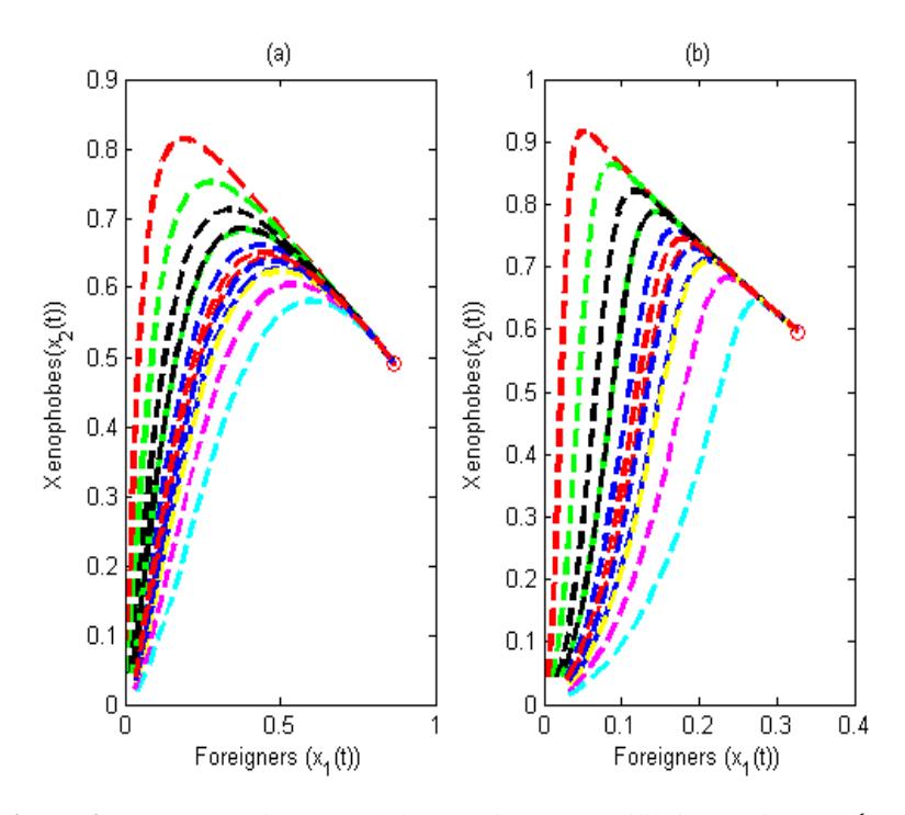
Figure 2 Phase portraits around the coexistence equilibrium point, 12(1 , 2 ) of Model (4) at different initial values.
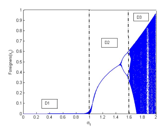
Figure 3 Bifurcation diagram of foreigners, 1 () for 1 ∈ [0, 2], 12 = 0.965 and initial values (0.1, 1). The stable domain, unstable domain and chaotic domain are denoted by 1 ,2 and 3 respectively.
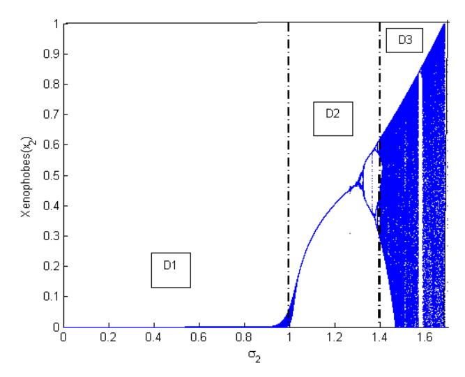
Figure 4 Bifurcation diagram of xenophobes, 2 () for 2 ∈ [0, 1.7], 21 = 0.65, = 1.5 and initial values (1, 0.9). The stable domain, unstable domain and chaotic domain are denoted by 1 ,2 and 3 respectively.
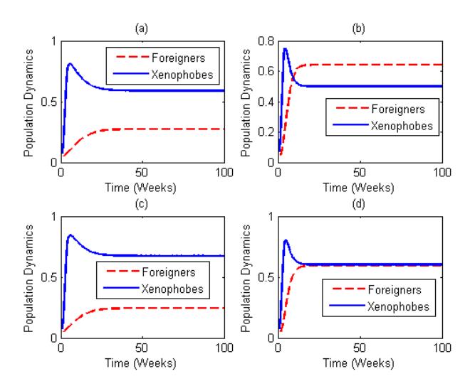
Figure 5 Plots displaying the population dynamics of foreigners and xenophobes when (a) = = 0; (b) = 0.8, = 0; (c) = 0, = 0.8 and (d) = 0.8, = 0.8 and initial values (0.025, 0.075).
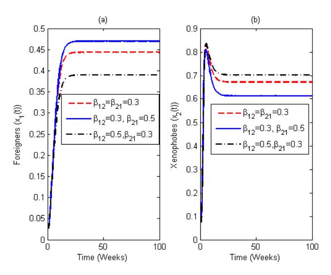
Figure 6 Population dynamics of foreigners and xenophobes when the attacking effect, 12 and retaliating effect, 21 are varied and other parameter values are kept constant with initial values (0.025, 0.075).
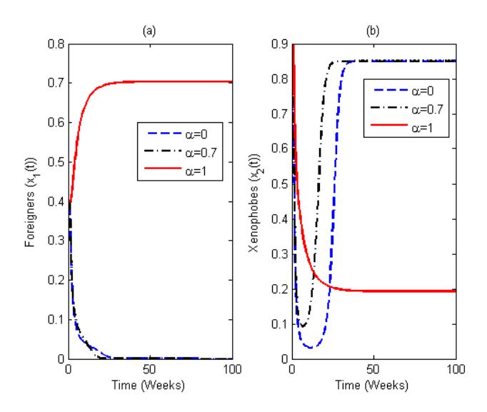
Figure 7 Population dynamics of foreigners and xenophobes for ∈ [0, 0.7, 1], 12 = 0.5, 1 = 200, 2 = 300, = 0.1, 1 = 0.2, 2 = 0.15 and initial values (0.4, 0.9).
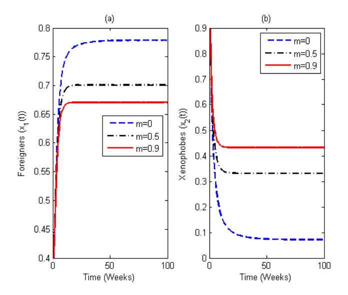
Figure 8 Population dynamics of foreigners and xenophobes for ∈ [0, 0.5, 0.9], 12 = 0.5,1 = 200,2 = 300, = 1, 1 = 0.2, 2 = 0.15 and initial values (0.4, 0.9).
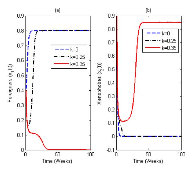
Figure 9 Population dynamics of foreigners and xenophobes ∈ [0, 0.25, 0.35], 12 = 0.5, 21 = 1, 1 = 200, 2 = 300, = 0.1, 1 = 0.2, 2 = 0.15, and initial values (0.4, 0.9).
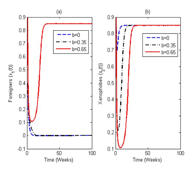
Figure 10 Population dynamics of foreigners and xenophobes ∈ [0, 0.35, 0.65], 12 = 0.5, 21 = 1, 1 = 200, 2 = 300, = 0.75, 1 = 0.2, 2 = 0.15, and initial values (0.4, 0.9).
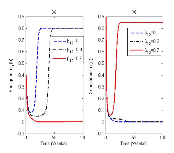
Figure 11 Population dynamics of foreigners and xenophobes for 12 ∈ [0, 0.3, 0.7], 21 = 1, 1 = 200, 2 = 300, = 0.1, 1 = 0.2, 2 = 0.15 and initial values (0.4, 0.9).
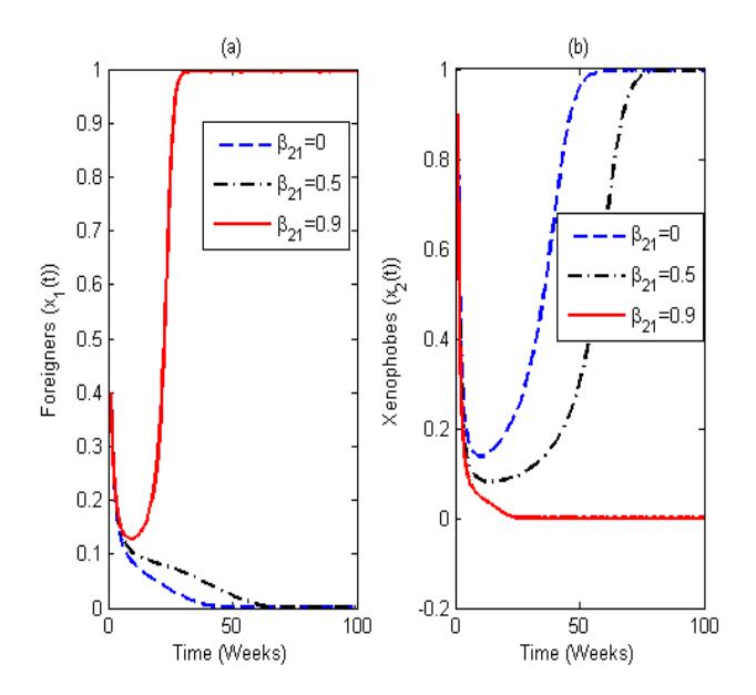
Figure 12 Population dynamics of foreigners and xenophobes for 12 ∈ [0, 0.5, 0.9], 12 = 0.3,1 = 200,2 = 300, 1 = 0.2, 2 = 0.15 and initial values (0.4, 0.9).
5 Discussion
We have shown numerically in Figure 3 and Figure 4 that the positive coexistence point of the system has period-doubling bifurcation, which is an indication that xenophobic attacks in Africa may lead to chaotic situations if immediate interventions are not offered. Nevertheless, we can see in Figure 5(a) and Figure 5(c) that when there is no group defense by foreigners, the xenophobes dominate the economy and take control of their resources. Meanwhile, Figure 5(b) describes the economic dominance of foreigners over xenophobes in the presence of high group defense against xenophobia. Figure 5(d) shows a state of coexistence between foreigners and xenophobes. This means both populations share stable economic prospects. In Figure 6, when the retaliating effect on xenophobes supercedes the attack rate (\(\beta_{12} < \beta_{21}\)), the population of foreigners grows economically while the population of xenophobes decreases. The converse situation is obtained for the case (\(\beta_{12}\) > \(\beta_{21}\)). But whenever (\(\beta_{12} = \beta_{21}\)), the highest economic peak for the xenophobe population is twice that of the foreigner population before achieving stability. Figure 7 shows that increasing the level of group defense encourage more foreigners to partake in business activities outside their country of origin and reduces the number of xenophobes fighting against them. Meanwhile antixenophobic policy also helps to reduce the number of xenophobes and creates room for more participation by foreigners in the economy, as clearly illustrated in Figure 8. The implication of this outcome is that a good security architecture combined with anti-xenophobic policies will protect and defend foreigners from xenophobic attacks and control subsequent incidences. From Figure 9, we note that for xenophobes to fight freely indeed depends on the level of fear of foreigners. That is, more fear in foreigners reduces their population density and increases that of xenophobes. In Figure 10 we can see that an increase in the tolerance level of both foreigners and xenophobes causes them to attain a stable population. On the other hand, increasing \(\beta_{12}\) and \(\beta_{21}\) respectively decreases the non-indigenous population and xenophobes, as shown in Figure 11 and Figure 12. Therefore, it becomes pertinent for the concerned nations to sign bilateral engagements that will end the consequences of xenophobia in Africa and the world at large. Like other mathematical models, our model too has some shortcomings. The parameter values on xenophobic attacks are hard to come by. Some were adopted for the purpose of illustration from the predator-prey study by Sasmal & Takeuchi [16]. As such it is unrealistic to promise ideal results from this paper.
6 Conclusion
The fight against xenophobic attacks just like infectious diseases is a challenge in Africa and the rest of the world. In this paper, we propose a mathematical
model of xenophobia in Africa using the principle of competitive exclusion in a predator-prey system. We non-dimensionalized the model to identify the fraction of foreigners that are prey to xenophobic attacks and the exact proportion of xenophobes that advance the phenomenon. The nondimensionalized model is mathematically characterized by a solution that is uniformly bounded. The model has four forms of equilibria with four different cases, namely the trivial state \((X_{00})\), the case when non-natives are banned completely from a foreign country; \((X_{02})\), the case when xenophobes are no more active \((X_{10})\); and the case when both populations coexist in a particular country \((X_{12})\). Apart from the trivial equilibrium, which is unstable, all other equilibrium states have been proved to be locally and globally stable with respect to the parametric conditions in Theorems 2, 3 and 4. In addition, this study revealed under the same conditions that each non-trivial equilibrium of the model undergoes transcritical bifurcation in Theorem 5. We also confirmed by numerical simulation that the model has period-doubling bifurcation, which is an indicator for chaotic situation of xenophobia in Africa. So far, based on our results, we can conclude that tolerance and anti-xenophobic policies could be important parameters for controlling the xenophobic crisis in Africa.
Acknowledgement
The authors would like to thank the anonymous referees for their invaluable comments and suggestions.