
1. Introduction
Cholera is an intense diarrhoeal infection. It is caused by the ingestion of contaminated food or water containing bacteria of the genus Vibrio cholerae. It is estimated that each year 2.9 million cases of cholera appear all around the world, causing 95,000 deaths. This malady is normally moderate but can sometimes be severe. Approximately 10% of affected people have severe infection, showing excessive diarrhea, vomiting and leg cramps. They may suffer rapid loss of body fluids, leading to dehydration and without treatment death can occur within hours [1].
Transmission of cholera disease is related to inappropriate access to safe drinking water and lack of healthy living conditions. Regions that include periurban ghettos and camps are at high risk of catching the disease because people do not have clean water and proper sanitation facilities there. The consequences of a humanitarian crisis can increase the risk of cholera transmission due to the exposure to cholera bacteria. Infected bodies as the source of an epidemic have never been reported [2]. According to WHO, cholera cases have continuously been increasing for several years. For instance, during 2017, almost 1,227,391 cases were reported from 34 countries, including 5,654 deaths [2].
The dynamics of cholera transmission include interactions such as human to host and pathogen to environment interactions. These contribute to horizontal transmission (human-human) and indirect (environment-human) transmission pathways. An individual may become infected with cholera through drinking water or eating food that is infected with cholera bacteria. The source of contamination during a cholera epidemic are usually water and food polluted by the excretions of infected people. Rapid spread of the disease occurs in areas in which sewage treatment and clean water supply are inadequate. Casual contact of an infected person with others does not spread the disease [3].
Even though cholera is a severe infection, it can be controlled by supplying clean water with satisfactory sterilization, proper treatment of patients and an adequate oral cholera vaccine [4]. In 2010, WHO urged the use of cholera vaccines in endemic environments and presumably during epidemics and emergency situations. The disease can usually be treated through oral rehydration salts and WHO has formally endorsed the use of these salts (sugar, salt and clean water), resulting in the prevention of 40 million deaths, as this strategy can reduce mortality rates below 1% when properly executed [5].
The cholera disease problem has been studied through different approaches. In mathematical modeling, in particular qualitative analysis of dynamical systems has been used for the understanding and prediction of infection behavior. Over time, numerous mathematical models describing the dynamics of cholera have been proposed and analyzed, see for instance [6]-[13]. Recently, some mathematical models have been formulated under the assumption of coinfection with other diseases, such as schistosomiasis [14], HIV [15] and malaria [16]. Additionally, optimal control theory has been an efficient tool for better understanding the complex dynamical system and its control. The most recent works can be found in references [17]-[19]. Regarding the control problem for cholera disease, we highlight the works reported in references [20]-[26].
In this work, we intended to comprehend the impacts of some control efforts coupled with different transmission pathways of cholera. We applied three control campaigns and analyzed the best combination of them. Furthermore, we determined the most cost-effective campaign for control by using the Incremental Cost-Effectiveness Rate (ICER). This attempt provided us with valuable rules for effective mitigation and intervention strategies against cholera epidemics. More specifically, we modified the model given in [20] by including
three sorts of controls: personal protection, drug treatment (hydration therapy, antibiotics and others), and water sanitation as functions of time. Then, we formulated a state-adjoint framework and inferred the essential conditions for the optimal control strategies. Numerical simulations were performed to analyze single and multiple controls. This analysis is expected to help planners plan efforts that must be made to avoid an increase in cholera cases.
2. Optimal Control Problem
Here, we propose the compartmental mathematical model of interaction between humans and cholera bacteria shown in Figure 1. With this model, we survey the effects of personal protection, drug treatment and water sanitation as control measures. The human population N(t) at time t is partitioned into seven compartments: susceptible (), educated (), vaccinated (), infectious (), quarantined (), treated (), and recovered (), Thus () = () + () + () + () + () + () + (), while the cholera bacteria in the aquatic reservoir population at time t is represented by the term B(t). We suppose that the human population is recruited at a rate Λ and dies naturally at a rate µ and both infected and treated individuals die due to infection at rates 1 and 2, respectively, with 1 ≥ 2. Therefore, the ordinary differential equation (ODE), which represents the evolution of human population over time, is:
\[\frac{dN(t)}{dt} = \Lambda - \mu N(t) - \sigma_1 I(t) - \sigma_2 T(t). \tag{1}\]
We also assume that the cholera bacteria population is recruited in the environment by logistic growth rate (1 − ), where n is the per capita development rate and is the carrying capacity of the environment. Each
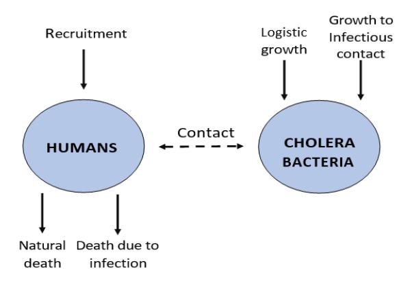
Figure 1 Compartmental diagram of interaction between humans and cholera bacteria.
infected individual contributes (cells/L-per day) to Vibro cholerae in the aquatic population with a fixed rate, e. Thus, the ODE representing the evolution of the bacteria population over time is:
\[\frac{dB(t)}{dt} = n\left(1 - \frac{B(t)}{K_B}\right)B(t) + eI(t). \tag{2}\]
Note that Eq. (1) and Eq. (2) are coupled. Now, we define the force of infection for susceptible, educated and vaccinated humans as \(\frac{\beta B}{H+B}\), where \(\beta\) represents the ingestion rate of Vibrio cholerae from contaminated sources and H is the concentration of vibrios in contaminated water. Then \(\frac{\beta B}{H+B}S\) represents the number of susceptible individuals that become infected, \(q(1-\tau)\frac{\beta B}{H+B}E\) is the number of educated individuals that become quarantined, where q is the failure of education rate, and \(\tau \in [0,1]\) is the efficacy of quarantine rate, and \(p\frac{\beta B}{H+B}V\) represents the number of vaccinated individuals that become infected, where p is the reduction of susceptibility rate due to vaccination. Other parameters involved in the model are specified in Table 1.
Table 1 Parameters Involved on Model Given on Eq. (3): Description, Units and Values Parameter.
| Symbol | Description | Dimension | Value | Reference |
|---|---|---|---|---|
| Λ | Recruitment rate of humans | Hum x Day−1 | 15.18535 | [20] |
| ω | Vaccine effectiveness loss rate | \(Day^{-1}\) | 0.003 | [20] |
| 3 | Not taking precautions rate | \(Day^{-1}\) | 0.003 | [20] |
| а | Temporary immunity loss rate | \(Day^{-1}\) | 0.003 | [20] |
| \(\psi\) | Education rate | \(Day^{-1}\) | 0.008 | [20] |
| ф | Vaccination rate | \(Day^{-1}\) | 0.07 | [20] |
| β | Infection rate for infected water consumption | \(Day^{-1}\) | 0.2143 | [27] |
| γ | Infection rate of educated individuals | \(Day^{-1}\) | 0.005 | [20] |
| ρ | Inefficacy of vaccine | Dimensionless | 0.15 | [28] |
| \(\sigma_1\) | Infection death rate of infected individuals | \(Day^{-1}\) | 0.015 | [27] |
| q | Failure rate of education | Dimensionless | 0.002 | [20] |
| θ | Transition rate from quarantined | \(Day^{-1}\) | 0.005 | [20] |
| α | Recovery rate due to treatment | \(Day^{-1}\) | 0.2 | [20] |
|---|---|---|---|---|
| \(\sigma_2\) | Infection death rate of treated individuals | \(Day^{-1}\) | 0.0001 | [20] |
| \(\varsigma_2\) | Efficacy of control by treatment | \(Day^{-1}\) | 0.34 | Assumed |
| ħ | Bacterial reproduction rate | \(Day^{-1}\) | 0.73 | [29] |
| \(K_B\) | Environmental carrying capacity | Bacteria | 107 | [30] |
| e | Contribution of infected individuals to the | \(Day^{-1}\) | 100 | [30] |
| \(\varsigma_3\) | Efficacy of control by water sanitation | Dimensionless | 0.54 | Assumed |
| μ | Natural death rate | \(Day^{-1}\) | 0.0185 | Assumed |
| δ | Treatment rate of infected individuals | \(Day^{-1}\) | 0.005 | [20] |
In order to reduce the burden of infection, we introduce the following control campaigns as functions depending on time (bang-bang controls [31]): \(u_1(t)\) represents control by personal protection through the use of clean water, \(u_2(t)\) is control by drug treatment of infected individuals including hydration therapy, and \(u_3(t)\) represents control by water sanitation, which leads to the death of bacteria. The expression \((1-u_1(t))\frac{\beta B}{H+B}\) indicates a kind of resistance to infection, where \(u_1(t)=1\) if the control by personal protection is 100% effective, i.e. there is no infection, while \(u_1(t)=0\) if the control is not effective. Similarly, the expressions \(\xi_2 u_2(t)I\) and \(\xi_3 u_3(t)B\) represent the number of infected individuals and bacteria reduced by the controls, where parameters \(\xi_i \in [0,1]\) with i=1,2 are the efficacy rates of the controls. The control variables \(u_i(t)\), with i=1,2,3 are in the set \(\mathfrak U\) of Lebesgue measurable functions on [0,1].
We can represent our control problem in terms of the following system of nonlinear ODEs:
\[\begin{cases} \min_{U \in \mathfrak{I}} J[U] = \int_{0}^{T} \left( A_{1}I + A_{2}B + \frac{1}{2} (B_{1}u_{1}^{2} + B_{2}u_{2}^{2} + B_{3}u_{3}^{2}) \right) dt \\ \frac{dS}{dt} = \Lambda + \omega V + \varepsilon E + aR - \left( \mu + \psi + \phi + \left( 1 - u_{1}(t) \right) \frac{\beta B}{H + B} \right) S \\ \frac{dE}{dt} = \psi S - \left( \mu + \varepsilon + \gamma + \left( 1 - u_{1}(t) \right) \frac{q\beta(1 - \tau)B}{H + B} \right) E \\ \frac{dV}{dt} = \phi S - \left( \omega + \mu + \left( 1 - u_{1}(t) \right) \frac{p\beta B}{H + B} \right) V \\ \frac{dI}{dt} = \theta Q + \gamma E + \left( \left( 1 - u_{1} \right) \frac{\beta B}{H + B} \right) S + \left( \left( 1 - u_{1} \right) \frac{p\beta B}{H + B} \right) V - \left( \xi_{2}u_{2} + \delta \mu + \sigma_{1} \right) I \end{cases}\] \[\begin{cases} \frac{dQ}{dt} = \left( 1 - u_{1}(t) \right) \frac{q\beta(1 - \tau)B}{H + B} E - \left( \theta + \mu \right) Q \\ \frac{dT}{dt} = \xi_{2}u_{2}I + \delta I - \left( \mu + \alpha + \sigma_{2} \right) T \\ \frac{dR}{dt} = \alpha T - \left( \alpha + \mu \right) R \\ \frac{dB}{dt} = \left( n \left( 1 - \frac{B}{K_{B}} \right) - m \right) B + eI - \xi_{3}u_{3}B \\ X(0) = \left( S(0), E(0), V(0), I(0), Q(0), T(0), R(0), B(0), \right) = X_{0} \\ X(T) = \left( S^{*}, E^{*}, V^{*}, I^{*}, Q^{*}, T^{*}, R^{*}, B^{*} \right) = X_{1}. \end{cases}\]
In the above optimal control problem, \(X_0\) represents the disease-free equilibrium (DFE) of the state equations, \(X_1\) is the endemic equilibrium of the state equation and \(U(t) = (u_1(t), u_2(t), u_3(t))\) is the vector of controls, which is subjected to the performance index (or cost function) \(J[\mathbf{U}]\). In the expression for J we have that \(A_1\) and \(A_2\) express the social costs depending on the number of individuals infected with cholera; \(B_1\), \(B_2\) and \(B_3\) represent absolute costs generated with the implementation of the controls; and T is the time of implementation of the control campaign.
Our main goal was to determine the necessary conditions for the existence of an optimal control \(U^*\) to reduce the number of infected individuals with the minimum cost. Our second objective was to validate the theoretical results with numerical experiments using data from the literature.
3. Theoretical Results
In this section, we use the classical results given in [32] and [33] to prove the existence of optimal controls. We should check that the following hypotheses are satisfied:
- 1. The set consisting of controls and corresponding described variables is non-empty and the set where the control U takes its values from is convex and closed.
- 2. The system of the state equations is bounded through a linear function in the state and control.
- 3. The integrand of the performance index J is convex on \(\mathbf{U}\) and is also bounded below by \(c_1(\sum_{i=1}^3 |u_i|)^{\frac{\beta}{2}} c_2\), where \(c_1\), \(c_2 > 0\) and \(\beta > 1\).
Hypotheses (1) and (2) are obviously satisfied. The last condition is also satisfied. In fact,
\[A_1I + A_2B + \frac{1}{2}(B_1u_1^2 + B_2u_2^2 + B_3u_3^2) \ge c_1(|u_1|^2 + |u_2|^2)^{\frac{\beta}{2}} - c_2,\] where, \(\beta > 1\) and \(A_1\), \(A_2\), \(B_1\), \(B_2\), \(B_3\), \(c_1\), \(c_2 > 0\). Thus, we have the following theorem:
Theorem 3.1 There is an optimal control \(U^* = (u_1^*, u_2^*, u_3^*)\) that satisfies Problem (3).
The optimal solution can be through the Lagrangian and Hamiltonian for the control problem (3). The Lagrangian is defined as:
\[L(I, B, u_1, u_2, u_3) = A_1 I + A_2 B + \frac{1}{2} B_1 u_1^2 + \frac{1}{2} B_2 u_2^2 + \frac{1}{2} B_3 u_3^2.\]
We have to find the minimal value of the Lagrangian. For this end, we define the Hamiltonian H for the control problem as:
\[\begin{split} H(X,U,\lambda) &= A_{1}I + A_{2}B + \frac{B_{1}}{2}u_{1}^{2} + \frac{B_{2}}{2}u_{2}^{2} + \frac{B_{3}}{2}u_{3}^{2} + \lambda_{1}\left(\Lambda + \omega V + \varepsilon E + aR - \left(\mu + \psi + \phi + (1 - u_{1})\frac{\beta B}{H + B}\right)S\right) + \\ \lambda_{2}\left(\psi S - \left(\mu + \varepsilon + \gamma + (1 - u_{1})\frac{q\beta(1 - \tau)B}{H + B}\right)E\right) + \\ \lambda_{3}\left(\phi S - \left(\omega + \mu + (1 - u_{1})\frac{p\beta B}{H + B}\right)V\right) + \lambda_{4}\left(\theta Q + \gamma E + \left((1 - u_{1})\frac{\beta B}{H + B}\right)S + \left((1 - u_{1})\frac{p\beta B}{H + B}\right)V - \\ (\xi_{2}u_{2} + \delta + \mu + \sigma_{1})I\right) + \lambda_{5}\left((1 - u_{1})\frac{q\beta(1 - \tau)B}{H + B}E - \frac{\beta B}{H + B}\right)I - \end{split}\]
\[\begin{split} &(\theta+\mu)Q\Big) + \lambda_6(\xi_2 u_2 I + \delta I - (\mu + \alpha + \sigma_2)T) + \\ &\lambda_7(\alpha T - (\alpha+\mu)R) + \lambda_8\bigg(\Big(n(1-\frac{B}{K_B}) - m\Big)B + eI - \\ &\xi_3 u_3 B\bigg), \end{split}\] where \(\mathbf{X} = (S, E, V, I, Q, T, R, B)\) and \(\lambda = (\lambda_1, \lambda_2, \dots, \lambda_8)\) is the vector of adjoint variables. We can summarize the main result of this section in the following theorem:
Theorem 3.2 There is an optimal solution, denoted by \(X^*(t)\), which minimizes J in [0, T], and a vector of adjoint variables \(\lambda\) such that
\[\begin{cases} \frac{d\lambda_{1}}{dt} = \lambda_{1}\mu + (\lambda_{1} - \lambda_{2})\psi + (\lambda_{1} - \lambda_{3})\phi + (\lambda_{1} - \lambda_{4})\left((1 - u_{1})\frac{\beta B}{H + B}\right) \\ \frac{d\lambda_{2}}{dt} = -\lambda_{1}\varepsilon + \lambda_{2}\mu + \lambda_{2}\varepsilon + (\lambda_{2} - \lambda_{4})\gamma + (\lambda_{2} - \lambda_{5})\left((1 - u_{1})\frac{\beta B}{H + B}\right) \\ \frac{d\lambda_{3}}{dt} = (\lambda_{3} - \lambda_{1})\omega + \lambda_{3}\mu + (\lambda_{3} - \lambda_{4})\left((1 - u_{1})\frac{\beta B}{H + B}\right) \\ \frac{d\lambda_{4}}{dt} = -A_{1} + (\lambda_{4} - \lambda_{6})\xi_{2}u_{2} + (\lambda_{4} - \lambda_{6})\delta + \lambda_{4}(\mu + \sigma_{1}) - \lambda_{8}e \\ \frac{d\lambda_{5}}{dt} = (\lambda_{5} - \lambda_{4})\theta + \lambda_{5}\mu \\ \frac{d\lambda_{6}}{dt} = (\lambda_{6} - \lambda_{7})\alpha + \lambda_{6}(\mu + \sigma_{2}) \\ \frac{d\lambda_{7}}{dt} = (\lambda_{7} - \lambda_{1})\alpha + \lambda_{7}\mu \\ \frac{d\lambda_{8}}{dt} = -A_{2} + (\lambda_{1} - \lambda_{4})\left((1 - u_{1})\frac{BH}{(B + H)^{2}}\right)S + (\lambda_{2} - \lambda_{5})\left((1 - u_{1})\frac{\beta BH}{(B + H)^{2}}\right)V - \\ \lambda_{8}(n - m - 2\frac{nB}{K_{B}} - \xi_{3}u_{3}), \end{cases}\] with transversality condition \(\lambda(T) = 0\), which satisfies
\[u_{1}^{*} = \max \left\{ \min \left\{ \frac{1}{B_{1}} \left( (\lambda_{4} - \lambda_{1}) \frac{\beta B}{H+B} S + (\lambda_{5} - \lambda_{2}) \left( \frac{q\beta(1-\tau)B}{H+B} E \right) + (\lambda_{4} - \lambda_{3}) \frac{p\beta B}{H+B} V \right) \right\}, 0 \right\}\] \[(5)\]
\[u_{2}^{*} = \left\{ \left\{ 1, \frac{1}{B_{2}} ((\lambda_{4} - \lambda_{6}) \xi_{2} I) \right\}, 0 \right\}\] \[u_{3}^{*} = \left\{ \left\{ 1, \frac{1}{B_{3}} (\lambda_{8} \xi_{3} B) \right\}, 0 \right\}.\]
Proof 1 The Pontryagin principle given on reference [34] guarantees the existence of an adjoint variables vector \(\lambda\) that satisfies
\[\dot{\lambda}_{i} = \frac{d\lambda_{i}}{dt} = -\frac{\partial H}{\partial X}\] \[\lambda_{i}(T) = 0, i = 1,2,...,8\] \[H(X, U^{*}, \lambda, t) = \max H(X, U^{*}, \lambda, t), U \in \mathfrak{U}.\] (6)
or equivalently
\[\begin{split} \dot{\lambda}_1 &= -\frac{\partial H}{\partial S}, \quad \lambda_1(T) = 0 \\ \dot{\lambda}_2 &= -\frac{\partial H}{\partial E}, \quad \lambda_2(T) = 0 \\ \dot{\lambda}_3 &= -\frac{\partial H}{\partial V}, \quad \lambda_3(T) = 0 \\ \dot{\lambda}_4 &= -\frac{\partial H}{\partial I}, \quad \lambda_4(T) = 0 \end{split}\] \[\text{[rumus tidak dapat ditampilkan dengan baik — lihat PDF asli]}\]
Putting the derivatives of H with respect to X in the above equations we get system given on Eq. (4). Finally, from the optimality conditions for the Hamiltonian, which are given by \(\frac{\partial H}{\partial U^*} = 0\), we obtain the characterization of controls given on Eq. (5).
4. Numerical Experiments
Now, we carry out some numerical experiments in order to show how the controls affect the solutions of our control problem. The forward fourth-order Runge Kutta method is used to solve the state equations for the initial conditions, whereas the backward fourth-order Runge-Kutta method is applied to solve the adjoint system given on Eq. (4), given that we have final values. For the control variables we use an initial guess. We assume that the control campaign is conducted for 120 days. We propose four different controls campaigns:
1. Campaign 1: personal protection and hydration therapy, simultaneously.
- 2. Campaign 2: personal protection and water sanitation, simultaneously.
- 3. Campaign 3: hydration therapy and water sanitation, simultaneously.
- 4. Campaign 4: the combination of the three controls, simultaneously.
Table 2 shows the values that we have assigned to the relative weights associated with the controls.
4.1 Campaign 1: Numerical Simulations ( ≠ and ≠ )
Here we use two controls: personal protection and hydration therapy, simultaneously. It is observed from Figure 2(a) that the number of infected individuals decreases to zero after 20 days, but they start to appear again after 70 days. From Figure 2(b) we can infer that we have to apply hydration therapy for 120 days with full effort, and personal protection can be done to some extent.
| Table 2 Parameter Values Associated with the Control Problem. | |||
|---|---|---|---|
| Parameter | Value Reference | ||
|---|---|---|---|
| Relative weight | 𝐴1 | 1 | Assumed |
| 𝐴2 | 5 | Assumed | |
| Social costs | 𝐵1 | 5 | Assumed |
| 𝐵2 | 7 | Assumed | |
| 𝐵3 | 9 | Assumed | |
| Effectiveness | 𝜁2 | 0.34 | Assumed |
| 𝜁3 | 0.54 | Assumed |
4.2 Campaign 2: Numerical Simulations ( ≠ and ≠ )
Personal protection combined with water sanitation seems an excellent control campaign at first glance, as can be seen from Figure 3(a), but after 70 days it is
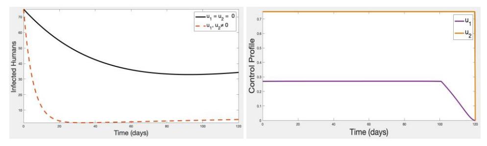
Figure 2 Trend of the number of infected humans under the implementation of Campaign 1 for (a) Infected individuals (left graph) and (b) Controls (right graph).
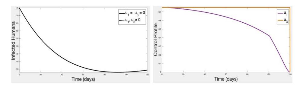
Figure 3 Trend of the number of infected humans under the implementation of Campaign 2 for (a) Infected individuals (left graph) and (b) Controls (right graph).
insufficient because infections start to appear again after this period. Figure 3(b) shows that water sanitation should be maintained for 120 days with full effort, however, personal protection may be decreased slowly.
4.3 Campaign 3: Numerical Simulations ( ≠ and ≠ )
When we use hydration therapy and water sanitation, we can see numerically that the effect starts to appear from the first day, because the number of infected individuals decreases and approaches to zero in 20 days, as shown by Figure 4(a). Figure 4(b) shows that these controls have to be fully applied for 120 days.
4.4 Campaign 4: Numerical Simulations ( ≠ , ≠ and ≠ )
In this campaign, we apply three controls: personal protection, hydration therapy and water sanitation. It can be observed from Figure 5(a) that the effect appears instantly as there is a high decrease in the number of infectious humans. After 15 days, the infection is eradicated completely. Figure 5(b) shows that we have to make a full effort for 120 days.
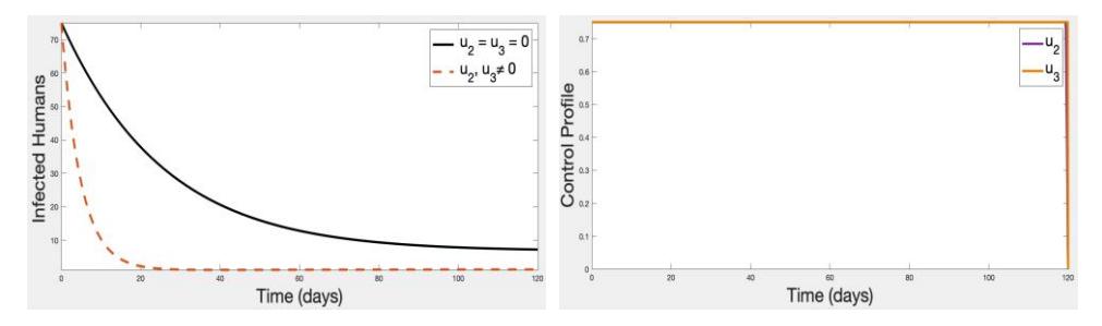
Figure 4 Trend of the number of infected humans under the implementation of Campaign 3 for (a) Infected individuals (left graph) and (b) Controls (right graph).
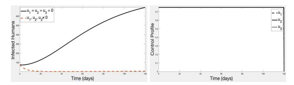
Figure 5 Trend of the number of infected humans under the implementation of Campaign 4 for (a) Infected individuals (left graph) and (b) Controls (right graph).
5. Cost-Effectiveness Analysis
In this section, we make an economic analysis of the control campaigns given in the previous section, in order to determine which is the most cost-effective campaign in controlling the cholera disease. Thus, we use the incremental costeffectiveness index (ICER), which is expressed in the following equation:
\[ICER = \frac{\Delta Cost}{\Delta Effect}. (7)\]
On the other hand, we want to quantify the cost-effectiveness of the control campaigns, for which we use the idea used in [35]. The ratio between number of Infections Avoided (IE) and Successful Recoveries (RE) is called the Index of Infections Avoided (IAR). It is defined as follows:
\[IAR = \frac{IE}{RE} \cdot \tag{8}\]
In the previous equation, the numerator represents the difference between the
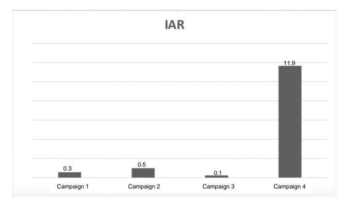
Figure 6 Comparison of the IAR of each control campaign.
total number of infectious individuals obtained by simulation without controls and the total number of infectious individuals obtained through simulations with controls. The calculation of the ICER values for each control campaign was done by means of Eq. (7). In Table 3 we show the highest IAR value for each control campaign.
Table 3 Index of Infections Avoided (IAR)
| Campaign 1 Campaign 2 | Campaign 3 | Campaign 4 | ||
|---|---|---|---|---|
| IE | 40 | 0.01 | 10 | 700 |
| RE | 70 | 0.01 | 40 | 60 |
| IAR | 0.571 | 1 | 0.25 | 11.66 |
From the above table we can conclude that the most cost-effective campaign in terms of IAR and total cost of intervention, is Campaign 4 (see Figure 6). Nevertheless, for more clarity, we examine the ICERs of each campaign. In Table 4, we show the classification of control campaigns defined by Eq. (3) in increasing order of effectiveness.
Table 4 ICER Comparison between Campaigns 2 and 3
| Campaign | Total avoided infections | Total cost | ICER |
|---|---|---|---|
| Campaign 2 | 0.01 | 2.3 | 230 |
| Campaign 3 | 10 | 3.1 | 0.08 |
| Campaign 1 | 40 | 2.5 | -2.395 |
| Campaign 4 | 700 | 1.9 | -1.896 |
The ICERs in Table 4 were computed as follows:
\[ICER(II) = \frac{2.3}{0.01} = 230\] \[ICER(III) = \frac{3.1 - 2.3}{10 - 0.01} = 0.08\] \[ICER(II) = \frac{2.5 - 3.1}{40 - 10} = -2.396\] \[ICER(IV) = \frac{1.9 - 2.5}{700 - 40} = -1.896\]
From Table 4 it can be concluded that Campaign 3 is 0.08 times less expensive than Campaign 2. Given that the ICER of Campaign 3 is smaller than that of Campaign 2, we can conclude that Campaign 2 is more expensive and less effective than Campaign 3. Therefore, we exclude it from the set of campaigns. Now, we recalculate the ICER indices of the remaining campaigns, as shown in Table 5.
Table 5 ICER Comparison between Campaigns 3 and 1
| Campaign | Total Avoided Infections | Total Cost | ICER |
|---|---|---|---|
| Campaign 3 | 10 | 3.1 | 0.31 |
| Campaign 1 | 40 | 2.5 | -2.396 |
| Campaign 4 | 700 | 1.9 | -1.896 |
From Table 5 and using an analogous reasoning to the previous one, we exclude Campaign 3 and recalculate the indices for a comparison between Campaigns 1 and 4. The results are shown in Table 6.
Table 6 ICER Comparison Between Campaigns 1 and 4
| Campaign | Total Avoided Infections | Total Cost | ICER |
|---|---|---|---|
| Campaign 1 | 40 | 2.5 | -0.0624 |
| Campaign 4 | 700 | 1.9 | -1.896 |
The results summarized in Table 6 coincide with the results given in Figure 6, where Campaign 4 has the highest IAR value because it has the lowest ICER value.
6. Conclusions
In this work, we approached cholera disease by mathematical modeling using ODEs, including some control strategies to understand the human bacteria transmission dynamics of the disease related to public health. We considered three sorts of controls in the form of personal protection, hydration therapy and water sanitation strategies. We used the previous control variables to formulate the optimal control problem in Eq. (3). Based on the three control variables we defined four control campaigns. The theoretical and numerical results showed that cholera disease can be controlled using any of these three campaigns. A cost-effectiveness analysis with data from the literature was carried out to determine the most cost-effective campaign.
It may be thought that applying three controls simultaneously could be very expensive and that it would be best to apply a single control or at most two of them simultaneously. However, the analysis evidenced that Campaign 3 (personal protection and water sanitation) and Campaign 4 (personal protection, hydration therapy, and water sanitation) were the cheapest options (at 2.3 and 1.9 units of cost, respectively). Additionally, these campaigns were the most effective in terms of the time required to reduce the incidence of cholera, with IAR indices of 1 and 11.66, respectively. Also, the differences between cost and health effects of the control campaigns were compared through ICER indices. For Campaign 4 we obtained the lowest index (-1.896), thus Campaign 4 is the most cost-effective campaign in controlling the cholera disease.
Although at present personal protection, hydration therapy and water sanitation should be guaranteed to all people, in some countries the desired conditions are not present. Some of the factors that influence the incidence and prevalence of cholera are lack of drinking water, lack of knowledge about the disease, and a high index of unsatisfied basic needs.
Acknowledgments
The authors would like to thank Miss. Rehana Farukh Ijaz, Assistant Professor, Department of the English, Government Associate College for Girls (Pakistan), who helped in improving the English of this manuscript. J. Romero thanks the support of Fundación Ceiba (Colombia).