
1 Introduction
Schistosomiasis is a neglected tropical disease that is associated with poor socioeconomic conditions such as lack of sanitation and treatment of infested waters [1]. It affects mostly children in communities where humans frequently come in contact with water bodies for socioeconomic activities. Schistosomiasis poses a serious public health challenge in many developing countries with incidence as high as one in thirty [2]. According to the WHO, an average of 206 million people worldwide took preventive treatment in 2016, while 89 million people received curative treatment [2]. Globally, schistosomiasis causes 200,000 deaths every year [3].
Schistosomiasis has a complex life cycle that is made up of two free living stages, miracidia and cercaria, the intermediate host, snail and the definitive host, man. The larva stage of schistosomiasis occurs when cercariae penetrate the skins of humans and develop into adult [4]. In a few weeks, these adult schistosomula produce eggs that are shed into the environment through urine and faeces by the definitive host. These eggs hatch in water and release miracidia, which penetrate the intermediate host dwelling in freshwater bodies. These miracidia develop into sporocysts inside the snails and asexual reproduction takes place after four weeks for the formation of cercariae. Shedding of these free living cercariae takes place by the infected snail, who swim and penetrate a new human host and the cycle continues. Schistosomiasis results from the host's immune response to schistosome eggs and granulomatous reactions [5]. The drug of choice for the treatment of schistosomiasis is praziquantel. The treatment leads to discontinuation of eggs deposition in the body, which averts its complications [6].
Some of the non-pharmacological interventions (NPI) advocated by the WHO include snail control and public health education. These NPI will complement the modern-day mass drug delivery programs for communities and school-age children for discontinuation of reinfection [7]. Snail control is the addition of molluscicides to water bodies that are frequently used by people and their livestock in day-to-day activities or for agricultural purposes [8]. Public health education strategy is about having adequate knowledge of the epidemiology of schistosomiasis. The majority of residents in endemic communities assume schistosomiasis is caused by soiltransmitted helminths, thus revealing their inadequate knowledge of the disease [9].
Mathematical modeling helps the understanding of the epidemiology of infectious diseases and also assists the decision making for public health policy formulation [10]. Mathematical modeling of schistosomiasis has been formulated in ordinary differential equations on several occasion and some researchers have developed new schistosomiasis models or modified existing ones using a deterministic approach [11]. Several models of schistosomiasis have been formulated with or without controls using different methods. Chiyaka & Garira [4] investigated the host-parasite dynamics of schistosomiasis, Ishikawa et al. [12] and Gurarie et al. [7] considered the effect of a mass treatment program with snail control, while Chiyaka et al. [13] observed that treatment eliminates the mature worms and active macrophages over a period of time with declining T-cell immune responses in the human body. The importance of public awareness campaigns was examined by Guiro et al. [14] and Yingke et al. [15], where Guiro et al. [14] used two general non-linear incidence functions and distributed delay. Diaby et al. [16] carried out a stability analysis of schistosomiasis dynamics, while Musa et al. [17] promoted the use of vaccination, and Ronoh et al. [18] considered the impact of environmental transmission in humans. Among the aforementioned authors, none discussed the importance of snail control and public health education for the dynamics of schistosomiasis. Also, there are only few works on modelling of schistosomiasis. Thus, the current work was aimed at evaluating the impact of public health education and snail control measures on schistosomiasis dynamics.
The rest of this paper is organized as follows. Section 2 presents the model formulation, while Section 3 provides an analysis of the model. The numerical simulations are in Section 4 and Section 5 contains the discussion and conclusion.
2 Model Formulation
The model traces the life cycle of the schistosome parasite at any time, t. The model is made up of human population, \(N_H(t)\); snail population, \(N_S(t)\); miracidia, M(t); and cercariae, C(t); at any time, t. The human population is subdivided into susceptible humans, \(S_H(t)\), acute infected humans, \(I_{1H}(t)\), and chronic infected humans, \(I_{2H}(t)\). Individuals in the human population move from one class to another as their status changes and as the disease evolves. Susceptible humans are humans without infection and have the ability to contract the disease when they come in contact with cercariae near fresh water. They progress to acute infected humans as a result of infection at rate \(\lambda_H\), where \(\lambda_H = \frac{\beta_H C(1-m)}{C_0 + \varepsilon C}\) and \(\beta_H\) is the transmission rate for cercariae to susceptible humans; \(m \in (0,1)\) is the public health education control strategy to reduce the transmission rate; \(C_0\) is the half saturation constant of cercariae in the environment; and \(\varepsilon\) is the limitation of the growth velocity of the parasite. The number of susceptible humans increases as a result of birth/immigration at rate \(\Lambda_H\) as well as acute infected humans that recover at rate e and return to the susceptible class, since re-infection is bound to occur as recovery does not result in permanent immunity. This takes place among humans in the acute infected class.
Acute infected humans recover when they take their treatment correctly. Those that miss or do not complete their treatment may progress to chronic infected humans at rate k. Chronic infected humans, \(I_{2H}(t)\), occur as a result of continuous deposition of parasite eggs in the human host. The human population dies naturally at rate \(\mu_H\), while the acute and chronic infected human subpopulations die of the disease at rates \(\sigma_{1H}\), and \(\sigma_{2H}\) respectively. We assume that disease-induced death of chronic infected humans is greater than that of acute infected humans, that is \(\sigma_{2H} > \sigma_{1H}\), since the complications of the chronic stage of the disease like liver and kidney failure as well as cancer and ectopic pregnancies may not allow recovery from the disease.
The acute and chronic infected humans, \(I_{1H}\) and \(I_{2H}\), shed eggs through their faeces and urine indiscriminately into the environment at rates \((1-m)\gamma_1\) and \(a(1-m)\gamma_1\), while public health education m reduces the shedding rate a becomes higher in the chronic stage. The shedding contributes to the life cycle of schistosoma. The eggs find their way into fresh water supplies and hatch into a free-swimming ciliated larva called miracidium, M. Miracidia, M, die naturally at rate \(\mu_M\) when there is no intermediate host (snail) to penetrate.
The snail population is subdivided into susceptible snail population \(S_S(t)\) and infected snail population \(I_S(t)\), at any time t. Recruitment into the susceptible snail class is by birth at rate \(\Lambda_S\), while the exit occurs as a result of disease infection when a susceptible snail comes in contact with miracidia, M, at rate \(\lambda_S\), or die naturally at rate \(\mu_S\), where \(\lambda_S = \frac{\beta_S M(1-\alpha b)}{M_0+\varepsilon M}\), and \(\beta_S\) is the transmission rate for miracidium to snails; \(\alpha \in (0,1)\) is snail control such the application of molluscicides or the hunting of snails; \(b \in (0,1)\) is the efficacy of the snail control; \(M_0\) is the half saturation constant of miracidia; and \(\varepsilon\) is the limitation of the growth velocity of the parasite larvae.
Snails that come in contact with water contaminated with miracidia get infected and progress to infected snails, \(I_S(t)\). We assume that the infected snails die of the disease at rate \(\sigma_S\). The infected snails release free living/swimming larvae called cercariae at rate \(\gamma_2\), of which the snail control \(\alpha\) reduces the shedding. The free-living larvae have the capacity to infect humans and die naturally at rate \(\mu_C\) in the absence of a human host. The contact patterns and snail population is assumed not to be affected by climatic variations. We also assumed that other animals such as cattle do not contribute to the parasite density in the environment. Also, there is neither vertical transmission of the disease in humans, nor immigration of infectious humans. In
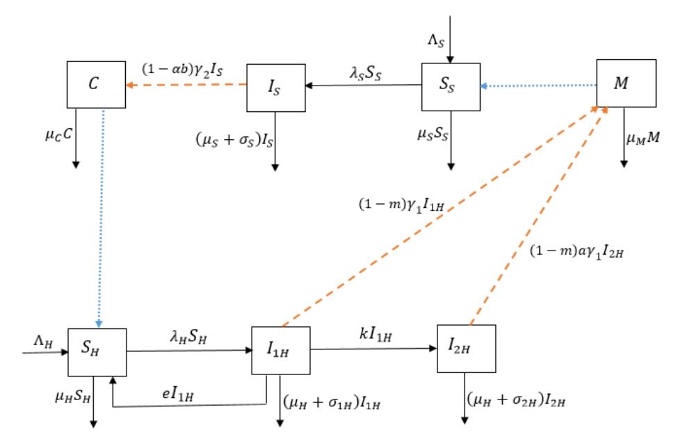
Figure 1 Schistosomiasis flow diagram. The blue dot arrow represents the interaction between susceptible humans and susceptible snails with the cercariae and miracidia respectively, while the orange dash arrow represents the shedding from infected humans and infected snails in the environment.
addition, infectious snails do not reproduce due to castration by the miracidia and seasonal variations do not affect snail populations and contact patterns. Furthermore, re-infection is bound to occur as infection does not result in permanent immunity [18]. This takes place among humans in the acute infected class.
Table 1 Model Parameters and Their Description
| Parameters | Description | Values (per day) | Sources |
|---|---|---|---|
| \(\Lambda_H\) | Recruitment rate for human population | 8000 | [4] |
| \(\Lambda_{S}\) | Recruitment rate for snail population | 200 | [4] |
| k | Progression rate from acute stage to chronic stage for human population | 0.05 | Assumed |
| \(\sigma_{1H}\) | Disease induced death rate for acute infected humans | 0.039 | [4] |
| \(\sigma_{2H}\) | Disease induced death rate for chronic infected humans | 0.05 | Assumed |
| e | Recovery rate for acute infected humans | 0.131 | Assumed |
| \(\mu_H\) | Natural death rate for human population | 0.0000384 | [4] |
| \(\mu_S\) | Natural death rate for snail population | 0.000569 | [4] |
| \(\beta_H\) | Transmission rate for human population | 0.406 | [4] |
| \(\beta_S\) | Transmission rate for snail population | 0.615 | [4] |
| m | Public health education parameter | [0,1] | Varied |
| \(\sigma_{ S}\) | Disease induced death for infected snail class | 0.0004012 | [14] |
| \(M_0\) | Half saturation constant of miracidia | \(1 \times 10^{8}\) | [4] |
| \(C_0\) | Half saturation constant of cercariae | \(9 \times 10^{7}\) | [4] |
| \(\gamma_1\) | Shedding rate for infected humans | 0.00232 | [4] |
| \(\gamma_2\) | Shedding rate for infected snails | 2.6 | [4] |
| а | Modification parameter of the shedding rate for chronic infected humans | 0.3 | Varied |
| α | Snail control parameter | [0,1] | Varied |
| b | Efficacy of the snail control parameter | [0,1] | Varied |
| \(\mu_C\) | Natural death rate for cercariae | 0.04 | [4] |
| \(\mu_{M}\) | Natural death rate for miracidia | 0.9 | [4] |
| ε | Growth velocity limitation of the pathogen | 0.2 | [4] |
A flow diagram of the model is presented in Figure 1 and a description of the parameters and their values and sources are given in Table 1.
From the description of the dynamics of schistosomiasis and the flow diagram in Figure 1, the following system of differential equations is derived:
\[\frac{dS_{H}}{dt} = \Lambda_{H} + eI_{1H} - \frac{\beta_{H}C(1-m)}{C_{0}+\varepsilon C}S_{H} - \mu_{H}S_{H}, \frac{dI_{1H}}{dt} = \frac{\beta_{H}C(1-m)}{C_{0}+\varepsilon C}S_{H} - eI_{1H} - kI_{1H} - (\mu_{H}+\sigma_{1H})I_{1H}, \frac{dI_{2H}}{dt} = kI_{1H} - (\mu_{H}+\sigma_{2H})I_{2H}, \frac{dM}{dt} = (1-m)\gamma_{1}I_{1H} + (1-m)\gamma_{1}aI_{2H} - \mu_{M}M, \frac{dS_{S}}{dt} = \Lambda_{S} - \frac{\beta_{S}M(1-\alpha b)}{M_{0}+\varepsilon M}S_{S} - \mu_{S}S_{S}, \frac{dI_{S}}{dt} = \frac{\beta_{S}M(1-\alpha b)}{M_{0}+\varepsilon M}S_{S} - (\mu_{S}+\sigma_{S})I_{S}, \frac{dC}{dt} = (1-\alpha b)\gamma_{2}I_{S} - \mu_{C}C,\] (1)
which is subject to initial conditions, (0) > 0, 1(0)≥ 0, 2(0)≥ 0, (0) ≥ 0, (0) > 0, (0)≥ 0 and C(0) ≥ 0. All model parameters are assumed to be positive.
3 Model Analysis
The basic properties of the model in Eq. (1) such as the invariant region, disease-free equilibrium state and its stability and basic reproduction number are discussed in this section.
3.1 Invariant region
The total human population at time , (), is given by
\[N_H(t) = S_H(t) + I_{1H}(t) + I_{2H}(t), (2)\] and the total snail population, (), is given by
\[N_S(t) = S_S(t) + I_S(t),\] (3)
with initial conditions (0) = 0, (0) = 0, C(0) = 0 ∗ and (0) = 0 ∗.
Theorem 1. The solutions of Eq. (1) will enter the positive invariant region, , that is uniformly bounded in a proper subset = × × × where = {(,1,2)ℝ+ 3 ∶ () ≤ Λ } is a subset of the human population, = {( , )ℝ+ 2 ∶ () ≤ Λ } is a subset of the snail population, = {() ≤ Λ (1−)2 } and = { () ≤ Λ1 (1−)(1+) } are subsets of cercariae and miracidia in the environment respectively.
Proof. Adding the human and snail subpopulations, we have
\[\frac{dN_H}{dt} = \Lambda_H - \mu_H N_H - \sigma_{1H} I_{1H} - \sigma_{2H} I_{2H} \text{ and } \frac{dN_S}{dt} = \Lambda_S - \mu_S N_S - \sigma_S I_S.\]
Without loss of generality, we assume that the dynamics of Eq. (1) without infection are asymptotically stable, that is, the disease-induced death rates for acute and chronic humans, \(\sigma_{1H}\) and \(\sigma_{2H}\) and infected snails, \(\sigma_{S}\), are negligible. So that, \(\frac{dN_{H}}{dt} \leq \Lambda_{H} - \mu_{H}N_{H}\) and \(\frac{dN_{S}}{dt} \leq \Lambda_{S} - \mu_{S}N_{S}\).
Applying the differential inequality theorem by Birkhoff & Rota [19] and integrating both sides of the equations with initial conditions \(N_H(0) = N_{H0}\) and \(N_S(0) = N_{S0}\), we have
\[N_H \le \frac{\Lambda_H}{\mu_H} - \left(\frac{\Lambda_H - \mu_H N_{H0}}{\mu_H}\right) e^{-\mu_H t} \,, \tag{4}\] and
\[N_S \le \frac{\Lambda_S}{\mu_S} - \left(\frac{\Lambda_S - \mu_S N_{S0}}{\mu_S}\right) e^{-\mu_S t}.\] (5)
As \(t \to \infty\) in Eqs. (4) and (5), the human and snail populations \(N_H\) and \(N_S\) approach \(N_H \le \frac{\Lambda_H}{\mu_H}\) and \(N_S \le \frac{\Lambda_S}{\mu_S}\) respectively. Thus, all feasible solutions of the human and snail populations enter the regions \(D_H = \left\{ (S_H, I_{1H}, I_{2H}) \in \mathbb{R}^3_+ : N_H(t) \le \frac{\Lambda_H}{\mu_H} \right\}\) and \(D_S = \left\{ (S_S, I_S) \in \mathbb{R}^2_+ : N_S(t) \le \frac{\Lambda_S}{\mu_S} \right\}\) respectively.
It is obvious that \(I_{1H} \leq N_H(t) \leq \frac{\Lambda_H}{\mu_H}\), \(I_{2H} \leq N_H(t) \leq \frac{\Lambda_H}{\mu_H}\) and \(I_S \leq N_S(t) \leq \frac{\Lambda_S}{\mu_S}\). With this, we rewrite the fourth and seventh equation of Eq. (1) for the miracidia and cercariae in the environment as
\[\frac{dM}{dt} \le \gamma_1 (1 - m)(1 + a) N_H(t) - \mu_M M \le \gamma_1 (1 - m)(1 + a) \frac{\Lambda_H}{\mu_H} - \mu_M M, \quad (6)\] and
\[\frac{d\mathcal{C}}{dt} \le (1 - \alpha b)\gamma_2 N_S(t) - \mu_C \mathcal{C} \le (1 - \alpha b)\gamma_2 \frac{\Lambda_S}{\mu_S} - \mu_C \mathcal{C}. \tag{7}\]
Using the differential inequality theorem by Birkhoff and Rota [19] on Eqs. (6) and (7), the miracidia M(t) and cercariae C(t), with \(M(0) = M_{0^*}\) and \(C(0) = C_{0^*}\) yield
\[M(t) \le \frac{\Lambda_H \gamma_1 (1 - m)(1 + a)}{\mu_H \, \mu_M} - \left( \frac{\Lambda_H \gamma_1 (1 - m)(1 + a) - \mu_H \, \mu_M M_{0^*}}{\mu_H \, \mu_M} \right) e^{-\mu_M t}. \tag{8}\] and
\[C(t) \le \frac{\Lambda_S(1-\alpha b)\gamma_2}{\mu_S \mu_C} - \left(\frac{(1-\alpha)\gamma_2 \Lambda_S - \mu_S \mu_C C_{0^*}}{\mu_S \mu_C}\right) e^{-\mu_C t}. \tag{9}\]
Thus, the miracidia and cercariae populations, \(M(t) \leq \frac{\Lambda_H \gamma_1 (1-m)(1+a)}{\mu_H \mu_M}\) and \(C(t) \leq \frac{\Lambda_S (1-\alpha b)\gamma_2}{\mu_S \mu_C}\) as \(t \to \infty\) in Eqs. (8) and (9) respectively.
Hence, the feasible solutions M(t) and C(t) will enter the positive invariant regions, \(D_M = \{ M(t) \le \frac{\Lambda_H \gamma_1 (1-m)(1+a)}{\mu_H \mu_M} \}\) and \(D_C = \{ C(t) \le \frac{\Lambda_S (1-\alpha b)\gamma_2}{\mu_S \mu_C} \}\). This completes the proof.
3.2 Existence and Stability of Disease-free Equilibrium State
3.2.1 Existence of the Disease-free Equilibrium State
The disease-free equilibrium state occurs at the state in which there is no infection, that is, \(I_{1H} = I_{2H} = I_S = C = M = 0\). Solving for the solutions of the system at equilibrium state, we have the disease-free equilibrium state, \(E_0\), given as \(E_0 = \left(\frac{\Lambda_H}{\mu_H}, 0, 0, 0, \frac{\Lambda_S}{\mu_S}, 0, 0\right)\). To carry out the local stability of the DFE, we first compute the basic reproduction number, \(R_0\).
3.2.2 Basic Reproduction Number, \(R_0\)
The basic reproduction number, \(R_0\), is the number of new cases reproduced in a wholly susceptible population when an infective individual is introduced into the population [20]. The important parameters as well as the transmission potentials of an infectious disease are emphasized by \(R_0\) [21]. When \(R_0 < 1\) it means that the disease will die out in the population, while \(R_0 > 1\) implies persistence of the disease in the population. \(R_0\) is computed using the next generation matrix approach by Van den Driessche & Watmough [20] at the disease-free equilibrium state, \(E_0\). The next generation matrix comprises of two parts: F and F0, where \(F = \left[\frac{\partial F_i(E_0)}{\partial x_j}\right]\) and F1 and F2 and F3. The functions, F3 and F4 are the new infections and the transfers of infections from one compartment to another respectively. F3 is the dominant eigenvalue or the spectral radius of the matrix, F3 with the associated matrix F3 and matrix F3 as the Jacobian matrices of F3 and F3 at F4 at F5 and F6 and F9. The next generation
The Jacobian matrices of \(F_i\) and \(V_i\) with respect to the infected state variables at \(E_0\) are given by approach is about the infected compartments, \(I_{1H}\), \(I_{2H}\), M, \(I_S\) and C.
\[\text{[rumus tidak dapat ditampilkan dengan baik — lihat PDF asli]}\] and
\[V = \begin{pmatrix} e + \mathbf{k} + \mu_H + \sigma_{1H} & 0 & 0 & 0 & 0 \\ -k & \mu_H + \sigma_{2H} & 0 & 0 & 0 \\ -(1-m)\gamma_1 & -(1-m)\alpha\gamma_1 & \mu_M & 0 & 0 \\ 0 & 0 & 0 & \mu_S + \sigma_S & 0 \\ 0 & 0 & 0 & -(1-\alpha b)\gamma_2 & \mu_C \end{pmatrix}.\]
The basic reproduction number, \(R_0\), which is the maximum positive eigenvalue of the matrix, \(FV^{-1}\), is given as
\[R_0 = \sqrt{R_{0S}R_{0H}} = \sqrt{\frac{\Lambda_S\Lambda_H\beta_S\beta_H\gamma_2\gamma_1 (g+ak)(1-m)^2 (1-\alpha b)^2}{(e+k+\mu_H+\sigma_{1H})(\mu_H+\sigma_{2H})(\mu_S+\sigma_S)C_0M_0\mu_C\mu_M\mu_H\mu_S}}\](10)
where
\[\begin{cases} R_{0HS} = R_{0HA} + R_{0HC}, \\ R_{0S} = \frac{\Lambda_S \beta_S \gamma_2 (1 - \alpha b)^2}{(\mu_S + \sigma_S) \mu_M \mu_S M_0}, \\ R_{0HA} = \frac{\Lambda_H \beta_H \gamma_1 g (1 - m)^2}{(e + k + \mu_H + \sigma_{1H}) (\mu_H + \sigma_{2H}) C_0 \mu_H \mu_C}, \\ R_{0HC} = \frac{\Lambda_H \beta_H \gamma_1 a k (1 - m)^2}{(e + k + \mu_H + \sigma_{1H}) (\mu_H + \sigma_{2H}) C_0 \mu_H \mu_C}. \end{cases}\](11)
The reproduction numbers \(R_{0S}\) and \(R_{0H}\) are the reproduction numbers that the snails and humans contribute through their respective shedding of miracidia and cercariae in the environment, while \(R_{0HA}\) and \(R_{0HC}\) are the reproduction numbers that the acute and chronic infected humans contributed by shedding miracidia in the environment respectively. Thus, for the disease to be controlled in the environment, the basic reproduction number, \(R_0\), should be less than unity, that is, \(R_0 < 1\), which means that \(R_{0HA}, R_{0HC} < \frac{1}{R_{0S}}\). This implies that the transmission rates for the human and snail populations satisfy the following inequalities: \(\beta_H^* < \frac{(e+k+\mu_H+\sigma_{1H})(\mu_H+\sigma_{2H})\mu_H\,\mu_M C_0}{\Lambda_H \gamma_1(\mu_H+\sigma_{2H}+ka)(1-m)^2}\) and \(\beta_S^* < \frac{(\mu_S+\sigma_S)\mu_S\mu_C\,M_0}{\Lambda_S\gamma_2(1-\alpha)^2}\).
3.2.3 Local stability of disease-free equilibrium
Local stability of the disease-free equilibrium is established using linearization, which is computes using the Jacobian matrix at disease-free equilibrium. We state the following theorem.
Theorem 2. The disease-free equilibrium, \(E_0\), is locally asymptotically stable whenever \(R_0 < 1\) and unstable if \(R_0 > 1\).
Proof. Using linearization method for the model in Eq. (1), the Jacobian matrix at the DFE, E<sub>0</sub>, is given as
\[J(E_0) = \begin{pmatrix} -\mu_H & e & 0 & 0 & 0 & 0 & -E \\ 0 & -f & 0 & 0 & 0 & 0 & E \\ 0 & k & -g & 0 & 0 & 0 & 0 \\ 0 & \gamma_1(1-m) & \alpha\gamma_1(1-m) & -\mu_M & 0 & 0 & 0 \\ 0 & 0 & 0 & -L & -\mu_S & 0 & 0 \\ 0 & 0 & 0 & L & 0 & -h & 0 \\ 0 & 0 & 0 & 0 & 0 & \gamma_2(1-\alpha b) & -\mu_C \end{pmatrix}\](12)
where
\[f = e + k + \mu_H + \sigma_{1H},\] \(g = \mu_H + \sigma_{2H},\) \(h = \mu_S + \sigma_{SS},\) \(E = \frac{S_B^0 \beta_H (1-m)}{C_0},\) \(L = \frac{S_S^0 \beta_S (1-\alpha b)}{M_0}.\)
The eigenvalues of the Jacobian matrix, \(J(E_0)\) are \(-\mu_S\), \(-\mu_S\) and the roots of the characteristic equation
\[\lambda^5 + A_1 \lambda^4 + A_2 \lambda^3 + A_3 \lambda^2 + A_4 \lambda^4 + A_5 = 0 \tag{13}\] where
\[\begin{split} A_1 &= f + \mu_M + \, \mathrm{g} \, + \, \mathrm{h} \, + \, \mu_C \, , \\ A_2 &= fg + fh + f\mu_C + f\mu_M + gh + g\mu_C + g\mu_M + h\mu_C + h\mu_M + \mu_C\mu_M , \\ A_3 &= fgh + fg\mu_C + fg\mu_M + fh\mu_C + fh\mu_M + f\mu_C\mu_M + gh\mu_C + gh\mu_M + g\mu_C\mu_M + h\mu_C\mu_M , \\ A_4 &= (1 - R_{0HC}R_{0S})fh\mu_M\mu_C + fgh\mu_C + fgh\mu_M + fg\mu_M\mu_C + g\mu_C\mu_M , \\ A_5 &= fgh\mu_M\mu_C (1 - R_0^2). \end{split}\]
Using the Routh-Hurwitz criterion, the roots of the characteristic Eq. (13) has negative real parts if the following inequalities are satisfied: i. \(A_1 > 0\), \(A_2 > 0\), \(A_3 > 0\), \(A_4 > 0\), \(A_5 > 0\), ii. \(A_1A_2 - A_3 > 0\), iii. \(A_3 (A_1A_2 - A_3) - A_4A_1^2 > 0\), iv. \(2A_1A_4 - A_2A_1^2 + A_2A_3\)
- \(A_5 > 0\). The inequalities ii, iii and iv are satisfied, provided \(A_i > 0\) ( i = 1, 2, 3, 4, 5) whenever \(R_0 < 1\). This is supported by the approach in Heffernan et al. [23]. Hence, the Jacobian matrix Eq. (13) has negative real eigenvalues if \(R_0 < 1\). Therefore, a local asymptotical stability exists for the disease-free equilibrium state whenever \(R_0 < 1\).
3.3 The Endemic Equilibrium State
The endemic equilibrium state, E, is the equilibrium state when there is infection in the population, that is, the infected variables are not equal to zero. Simultaneously solving the model in Eq. (1) at equilibrium state and simplifying yields the endemic equilibrium \(E_e = S_H^e, I_{1H}^e, I_{2H}^e, M^e, S_S^e, I_S^e, C^e\)), where
\[\begin{split} S_{H}^{e} &= \frac{H\Lambda_{H}\gamma_{1}(ak+g) - (k+\mu_{H} + \sigma_{1H})fghC_{0}M_{0}\mu_{C}\mu_{M}\mu_{H}\mu_{S}(R_{0}^{2} - 1)}{\mu_{H}\gamma_{1}(ak+g)H}, \\ I_{1H}^{e} &= \frac{fghC_{0}M_{0}\mu_{C}\mu_{M}\mu_{H}\mu_{S}(R_{0}^{2} - 1)}{\gamma_{1}(g+ak)H}, & I_{2H}^{e} &= \frac{kfghC_{0}M_{0}\mu_{C}\mu_{M}\mu_{H}\mu_{S}(R_{0}^{2} - 1)}{\gamma_{1}(g+ak)gH}, \\ M^{e} &= \frac{fghC_{0}M_{0}\mu_{C}\mu_{M}\mu_{H}\mu_{S}(R_{0}^{2} - 1)}{gH\mu_{M}}, & S_{S}^{e} &= \frac{Q\Lambda_{S}\gamma_{2} - fghC_{0}M_{0}\mu_{C}\mu_{M}\mu_{H}\mu_{S}(R_{0}^{2} - 1)}{\mu_{S}\gamma_{2}Q}, \\ I_{S}^{e} &= \frac{fghC_{0}M_{0}\mu_{C}\mu_{M}\mu_{H}\mu_{S}(R_{0}^{2} - 1)}{h\gamma_{2}Q}, & C^{e} &= \frac{fghC_{0}M_{0}\mu_{C}\mu_{M}\mu_{H}\mu_{S}(R_{0}^{2} - 1)}{hQ\mu_{C}} \end{split}\] with
\[H = (k + \mu_H + \sigma_{1H})\beta_S \Lambda_S \beta_H \gamma_2 + f \Lambda_S \beta_S \gamma_2 \mu_H \varepsilon + f h \varepsilon C_0 \mu_C \mu_H \mu_S + f h C_0 \beta_S \mu_C \mu_H\] \[Q = (ak + g)\beta_H \Lambda_H \gamma_1 (\mu_S + \beta_S) + f g \varepsilon M_0 \mu_H \mu_M \mu_S + (k + \mu_H + \sigma_{1H}) g M_0 \beta_H \mu_M \mu_S\]
This shows that an endemic equilibrium state \(E^e\) exists whenever \(R_0 > 1\).
3.3.1 Local stability of endemic equilibrium
The center manifold theory by Castillo-Chavez & Song [24] is used to establish the stability of the endemic equilibrium by proving the existence of forward bifurcation. The existence of forward bifurcation means that the disease-free and endemic equilibrium states are locally asymptotically stable if \(R_0 < 1\) and \(R_0 > 1\) respectively [22].
Using the center manifold theory [24], a forward bifurcation occurs at bifurcation parameter \(\phi = 0\) if the coefficient constants p < 0 and q > 0, otherwise there is backward bifurcation.
Solving for p and q, let \(\beta_S\) be the bifurcation parameter at \(R_0 = 1\) such that
\[\beta_S^* = \frac{fgh\mu_H\mu_M\mu_C\mu_S}{\Lambda_S\Lambda_H\beta_H\gamma_2\gamma_1(g+ak)(1-m)^2(1-\alpha b)^2}\] which implies that the Jacobian matrix in Eq. (12) has a simple zero eigenvalue and negative eigenvalues. This is proven in Theorem 2 using Routh-Hurwitz criterion and Heffernan et al.[23]. The right and left eigenvectors, \(w_i s\) and \(v_k s\), associated with the Jacobian matrix Eq. (12) at \(R_0 = 1\) are given by \(\mathbf{w} = (w_1, w_2, w_3, w_4, w_5, w_6, w_7)\) and \(\mathbf{v} = (v_1, v_2, v_3, v_4, v_5, v_6, v_7)\) where
\[\begin{split} w_1 &= -\frac{(\mathbf{k} + \mu_H + \sigma_{1H})}{\mu_H} w_2, & w_2 &= w_2 > 0, & w_3 &= \frac{k}{g} w_2, \\ w_4 &= \frac{\gamma_1 (1 - m)(g + ak)}{\mu_M} w_2, & w_5 &= \frac{L\gamma_1 (m - 1)(g + ak)}{\mu_M \mu_S} w_2, \\ w_6 &= \frac{L\gamma_1 (1 - m)(g + ak)}{h\mu_M} w_2, & w_7 &= \frac{f}{E} w_2, \\ v_1 &= 0, & v_2 &= v_2 > 0, \\ v_3 &= \frac{ahE\gamma_1\gamma_2 (1 - m)(1 - ab)}{g\mu_M \mu_C} v_2, & v_4 &= \frac{E\gamma_2 (1 - ab)}{\mu_M \mu_C} v_2, & v_5 &= 0, \\ v_6 &= \frac{E\gamma_2 (1 - ab)}{h\mu_C} v_2, & v_7 &= \frac{E}{\mu_C} v_2. \end{split}\]
Representing \(S_H = x_1\), \(I_{1H} = x_2\), \(I_{2H} = x_3\), \(M = x_4\), \(S_S = x_5\), \(I_S = x_6\), \(C = x_7\) in Eq. (1), we have non-zero second partial derivatives at DFE, \(E_0\), given by \(\frac{\partial^2 f_2}{\partial x_1 \partial x_7} = \frac{\beta_H (1-m)S_H^0}{C_0}\), \(\frac{\partial^2 f_2}{\partial x_7^2} = \frac{-2\varepsilon\beta_H \Lambda_H (1-m)S_H^0}{\mu_H C_0^2}\), \(\frac{\partial^2 f_6}{\partial x_4 \partial x_5} = \frac{\beta_S (1-\alpha b)S_S^0}{M_0}\), \(\frac{\partial^2 f_6}{\partial x_4^2} = \frac{-2\varepsilon\beta_S \Lambda_S (1-\alpha b)S_S^0}{\mu_S M_0^2}\), \(\frac{\partial^2 f_2}{\partial x_7 \partial \phi} = \frac{\varepsilon\Lambda_H (1-m)S_H^0}{\mu_H C_0^2}\), \(\frac{\partial^2 f_6}{\partial x_4 \partial \phi} = \frac{\varepsilon\Lambda_S (1-\alpha b)S_S^0}{\mu_S M_0^2}\).
The coefficient constants, p and q, are given by
\[\begin{split} p &= v_2 \left( w_1 w_7 \frac{\partial^2 f_2}{\partial x_1 \partial x_7} + w_7^2 \frac{\partial^2 f_2}{\partial x_7^2} + w_4 w_5 \frac{\partial^2 f_6}{\partial x_4 5} + w_4^2 \frac{\partial^2 f_6}{\partial x_4^2} \right) \\ &= -v_2 w_2^2 (1-m) \left[ \frac{f \beta_H S_H^0}{E C_0} \left( \frac{(k+\mu_H + \sigma_{1H}) C_0 + 2 \epsilon \mu_H \Lambda_H}{\mu_H C_0} \right) + E \gamma_2 \beta_S S_S^0 (1-m) (1-\alpha b)^2 (g+ak)^2 \gamma_1^2 \left( \frac{M_0 + 2 \epsilon \Lambda_S \mu_M}{\mu_M M_0} \right) \right] < 0, \\ q &= v_2 w_7 \frac{\partial^2 f_2}{\partial x_7 \partial \phi} + v_6 w_4 \frac{\partial^2 f_6}{\partial x_4 \partial \phi} \\ &= v_2 w_2 (1-m) \varepsilon \left[ \frac{f \Lambda_H S_H^0}{E \mu_H C_0} + \frac{(1-\alpha b)^2 (g+ak) \gamma_1 \Lambda_S S_S^0}{h \mu_C \mu_M \mu_S M_0^2} \right] > 0. \end{split}\]
We have the coefficients p < 0 and q > 0 since \(m, b, \alpha \in (0,1)\). The central manifold theorem implies that a forward bifurcation exists at \(R_0 = 1\) and \(\beta_S = \beta_S^*\). Hence, we can state the following theorem.
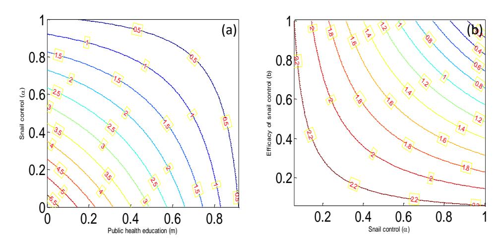
Figure 2 Contour plot for the basic reproduction number, \(R_0\), as (a) a function of snail control \((\alpha)\) and public health education (m), (b) a function of snail control \((\alpha)\) and the efficacy of the snail control (b). Here, the parameter values used are in the simulation were taken from Table 1.
Theorem 6. The endemic equilibrium point \(E^e\) of Eq. (1) is locally asymptotically stable when \(R_0 > 1\).
4 Numerical Simulations
The effects of snail control and public health education on the basic reproduction number, \(R_0\), is presented in Figure 2. System in Eq. (1) is solved numerically using the 4th-order Runge-Kutta's method and the solutions for the infected state variables are shown graphically in Figure 3. It shows the dynamics of each of the infected compartments. The parameter values used in the simulation were taken from Table 1.
5 Discussion
In Figure 2(a), the two control measures are implemented simultaneously and the basic reproduction number, \(R_0\), lies at their point of intersection. The basic reproduction number, \(R_0\), is less than unity under two conditions: when the public health education implementation is high (m = 0.8) and the snail control is low (\(\alpha = 0.3\)) on the one hand, and when public health education implementation is moderate (m = 0.6) and snail control is massive (\(\alpha = 0.8\)) on the other hand. Each of these has the potential of controlling the spread of schistosomiasis in the population. However, we advocate combined implementation of massive public health education and low level of snail control because it is more cost effective. This is important because it will avoid expensive and negative impacts that massive snail control will have on biodiversity. Figure 2(b) assesses the efficacy of snail control (molluscicide). From the figure, the efficacy of snail control must be very high ( ≥ 0.9) for the basic reproduction number to be less than unity. This implies that snail control works alongside public health education only if molluscicide application highly efficacious. In other words, even though the snail control coverage can work when it is low, as can be seen in Figure 2(a), the snail control must be highly efficacious in order to be able to halt the transmission of schistosomiasis.
Figure 3(a) and Figure 3(b) show the impacts of the control measures on the acutely and chronically infected human populations respectively under varying values of the control parameters. The behavior of the graphs (Figure 3(a) and Figure 3(b)) are similar in both instances. For instance, the basic reproduction number is less than unity (0 = 0.432,0 = 0.853 ) in each graph when there is massive coverage of public health education ( = 0.8) and the snail control is either 0.7 or 0.3 with an efficacy of 0.9. In Figure 3(c), the impact of the control parameters on the infected snail population with different values of control parameters is shown. Again, it can be seen that the basic reproduction number is less than unity (0 = 0.432,0 = 0.853) when public health education is 0.8 and snail control is either 0.7 or 0.3 with an efficacy of 0.9. Similar patterns can be observed in Figure 3(d) and Figure 3(e) where we considered the effect of the implementation of the control parameters on the concentrations of miracidia and cercariae in the environment respectively.
The findings in Figure 3(a) and Figure 3(b) imply that the number of people infected in the community will be reduced and ultimately lead to the control of schistosomiasis when there is combined implementation of massive public health education and either high or low coverage of environments infested with snails with highly efficacious molluscicide. Furthermore, the spread of schistosomiasis will also be halted when the concentrations of the infective stages of larvae (miracidia and cercariae) in the environment that infect snails and humans are reduced, as shown in Figure 3(d) and Figure 3(e) respectively. Thus, fewer snails and humans will be infected as the concentrations of miracidia and cercariae are reduced following the combined implementation of public health education and highly efficacious snail control.
A significant finding in this work is the pivotal role of public health education of the affected population in controlling the spread of schistosomiasis. This is because as more people become knowledgeable about the transmission of the disease, they will take measures to prevent being infected. Another significant finding is that a moderate coverage of the environment where snails live with highly efficacious molluscicide will reduce the transmission of the disease. We advocate the implementation of low coverage with highly efficacious molluscicide and massive public health education because it will lessen the negative effects of molluscicide on the biological role of snails in the ecosystem.
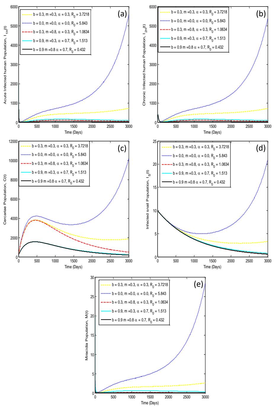
Figure 3 The impact of control strategies on schistosomiasis dynamics for the infected state variables, (a) \(I_{1H}(t)\), (b) \(I_{2H}(t)\), (c) C(t), (d) \(I_S(t)\), (e) M(t).
The findings in this work are in agreement with the recommendation by the WHO that public education and snail control should be implemented in order to achieve the control of schistosomiasis in affected communities. It will also aid public health professionals and policy makers in formulating control measures to reduce the transmission of the disease in the endemic population. Therefore, it is advocated that government agencies and non-governmental organizations should ensure that massive public health education and highly efficacious snail control (molluscicide) are implemented concurrently in order to halt the transmission of schistosomiasis among affected populations.
6 Conclusion
A mathematical model for the transmission dynamics of schistosomiasis was formulated in this work. The model was divided into human and snail sub-populations and their sheddings, miracidia and cercariae. Non-pharmacological interventions (NPIs) such as public health education and snail control were taken into consideration in this study. The basic reproduction number, 0, was computed and used to show its importance in achieving local stability of the disease-free equilibrium state when 0 < 1. The existence and stability of the endemic equilibrium state are established when 0 > 1. The stability of the endemic equilibrium was determined using the center manifold theory to prove forward bifurcation. Through numerical simulations it was observed that creating massive awareness of schistosomiasis among communities and implementation of widespread snail control in the environment with highly efficacious molluscicide will minimize the number of persons infected in the population. However, spraying of molluscicide in the environment (water bodies) on a massive scale may pose serious problem to biodiversity with huge cost implications. Therefore, it is recommended that the focus should be on implementing massive public health education and low-coverage snail control in endemic communities since this will also lead to the eradication of the disease.