
1 Introduction
Dengue Hemorrhagic Fever (DHF), or Dengue, is an infectious disease that is a serious global health threat. Dengue is caused by one of four different Dengue viruses and is transmitted from bites by infected female mosquitoes, mainly from Aedes aegypti and Aedes albopictus [1,2].
Dengue is a significant cause of death for children in Asian countries [3]. Since Dengue was first discovered in Indonesia in 1968 it has been the country with the most Dengue cases in Southeast Asia [1]. Based on data from Wahyudi et
al. [4], the number of Dengue cases in Indonesia is on the rise. From January 1 to March 4, 2020, 82 deaths and 14,716 cases were recorded. In March 2020, an outbreak of Dengue was reported in the Belitung Regency (Bangka Belitung Islands) and Sikka Regency (NTT). DKI Jakarta was among the five provinces in Indonesia with the highest number of Dengue incidents from 2011 to 2013 [5]. In short, the potential for Dengue outbreaks in DKI Jakarta deserves serious attention.
As a tropical country, Indonesia is an ideal place for mosquito breeding [6,7]. Climate change and community behavior are also important factors in influencing Dengue incidence [6]. In heavy monsoon conditions, the number of Dengue victims increases. Conversely, a decrease in the frequency of rain leads to a decrease in the number of Dengue incidents [6]. According to Pangribowo, et al. in [7], climate change can affect rainfall, temperature, humidity, and wind direction. Hence, it can affect the breeding patterns of Aedes mosquitoes.
Aedes mosquitoes thrive at an average temperature between 25 °C and 27 °C [8]. A relative humidity of more than 60% can increase metabolic processes in adult mosquitoes and prolong their lifespans. Rainfall also directly affects the incidence of Dengue by increasing the mosquito population due to the formation of large pools of stagnant water [9,10].
We strongly suspect there are links between weather characteristics and the Dengue incident rate in DKI Jakarta. To examine these links, we used clustering methods. Studies on various topics have been conducted using time-series clustering. Niennattrakul & Ratanamahatana [11] used K-means clustering with the DTW method on a leaf dataset. In addition, Hautamaki, et al. [12] researched three datasets from the UCI Machine Learning Repository, including hand-written characters, speech, and synthetic data. Furthermore, some analysis involves comparison of clustering methods with or without a time-series data structure, for example, Shobha & Asha [13] on meteorological data used Kmeans and hierarchical clustering without time-series data.
The use of cluster analysis to study Dengue has previously been done in other countries, such as Pakistan [14] and Singapore [15]. Also, a study has been conducted by Hariyanto & Shita [16] to determine the potential spread of Dengue by applying the K-Means clustering algorithm and Euclidean distance. Research on the relationships between weather factors and Dengue incidence using correlation analysis is reported by Hasanah & Susanna [17]. The results showed that Dengue incidence was significantly related to rainfall. The research by Tomia, et al. [5] in Ternate from 2007 to 2014 revealed that temperature was related to Dengue incidence, whereas rainfall and humidity were not.
The current research performed cluster analysis to obtain similarities and relationships between weather variables and Dengue incidence in DKI Jakarta. We used clustering on time-series and non-time-series data for DKI Jakarta from January 2008 to September 2017. The methods used were K-Medoids and Fuzzy C-Means (FCM) Clustering. Using both approaches, we hoped to better understand the relationships and similarities between all variables. The weather variables considered consisted of average temperature, rainfall, average relative humidity, average sunshine, and average wind speed.
The selection of the K-Medoids clustering method was based on the research conducted by Mohibullah, et al. [18]. According to Kaufman & Rousseeuw [19], the medoid makes the method able to cope more easily with outliers. We used FCM since it is reasonably accurate in determining the centroid of each cluster and in clustering data objects that are far apart from a solid cluster [20]. FCM is also able to cluster large amounts of data and is more robust against outliers. Dynamic Time Warping (DTW) distance was used for time-series clustering, while Euclidean distance was used for non-time-series clustering. The rest of this paper is organized as follows: Section 2 contains materials and methods, Section 3 contains the result, Section 4 contains the discussion, and finally, Section 5 contains the conclusion.
2 Materials and Methods
We first gathered a set of data from the DKI Jakarta Health Department [21], which included information on daily Dengue incidence in DKI Jakarta from January 1, 2008, to September 30, 2017. We obtained a second set of data from the Meteorology, Climatology, and Geophysical Agency (BMKG), which included daily weather information for five regions of DKI Jakarta: North Jakarta, Central Jakarta, South Jakarta, West Jakarta, and East Jakarta from January 1, 2008, to December 31, 2018. The Regency of Thousand Islands was not included in the dataset. For East Jakarta, the only available weather variables were rainfall, average relative humidity, and average temperature. For the other four regions, average sunshine and average wind speed were also available. As the data for 2008 contained many missing values, we restricted our study from December 30, 2008, to January 2, 2017.
We divided our research into clustering with time-series properties of the data taken into consideration (which we will refer to as time-series data) and clustering with time-series properties of the data ignored (which we will refer to as non-time-series data). Preprocessing consisted of several stages: selecting the variables used, data cleaning, data imputation, changing time to weekly for time-series clustering and yearly for non-time-series clustering, and data normalization. At this stage, the data used spans from 2009 to 2016. We then used K-Medoids and FCM Clustering to obtain our results. After preprocessing, data visualization was performed to illustrate the properties of each weather variable.
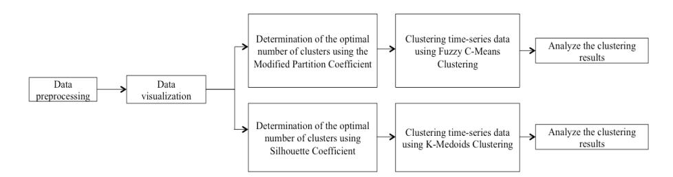
Figure 1 Flowchart of the research method on the time-series data.
For the time-series clustering approach, we clustered all the weather variables available for each region and the Dengue incidence variable as a weekly timeseries. Calculating the Silhouette Coefficient and the Modified Partition Coefficient (MPC) determines the optimal number of clusters when using K-Medoids and FCM, respectively. A flowchart of our research method for timeseries clustering is given in Figure 1. For the non-time-series clustering, we clustered the five regions in DKI Jakarta based on their similarity in weather and incidence characteristics. A flowchart of our research method for non-timeseries clustering is shown in Figure 2.
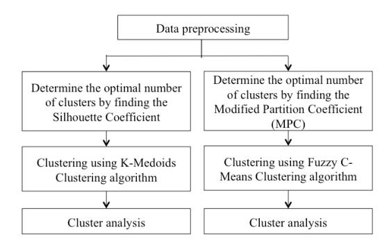
Figure 2 Flowchart of the research method on non-time-series data.
As previously explained, there were only three weather variables available for East Jakarta while there were two more weather variables for the other four regions. To be consistent, we used only three weather variables for non-timeseries clustering (rainfall, average relative humidity, average temperature), and the Dengue incidence variable.
2.1 Clustering Algorithms
Clustering is the process of grouping some objects into clusters so that similar objects in each cluster are distinct from objects in other clusters [22]. Timeseries clustering is a clustering algorithm for handling dynamic data and is useful for finding patterns in time-series datasets.
The Dynamic Time Warping (DTW) technique finds the optimal warping path between two time-series by stretching or shrinking its time axis [23]. An optimal warping path is one that minimizes the alignment between two timeseries. DTW is a shape-based similarity measure often used for time-series data, capable of handling such data of different lengths. Suppose we have two timeseries and with lengths and respectively as follows:
\[x = x_1, x_2, \dots, x_n; \ y = y_1, y_2, \dots, y_m.\] (1)
From the two time series in Eq. (1), the optimal warping path is determined using dynamic programming as follows: first, create an × cost matrix and for = 1,2, … , and = 1,2, … , , let , = | − | be the distance between and . We then set 1,1 = 1,1. Afterward, every other element , of the cost matrix is recursively defined by the following formula:
\[D_{i,j} = \begin{cases} L_{i,j} + D_{i,j-1}, & i = 1, \\ L_{i,j} + D_{i-1,j}, & j = 1, \\ L_{i,j} + \min\{D_{i-1,j}, D_{i,j-1}, D_{i-1,j-1}\}, & \text{otherwise.} \end{cases}\] (2)
The DTW distance between time-series and is defined as
\[DTW(\mathbf{x}, \mathbf{y}) = D_{n,m},\tag{3}\] while the optimal warping path is the path from (, ) to (1,1) formed by successively choosing either ( − 1,), (, − 1), or ( − 1, − 1) according to which one of −1, , ,−1, −1,−1 is the minimum as in Eq. (2). If (,) is contained in the optimal warping path, we can assume a connection between data points and .
We use the DTW distance when clustering the time-series data and the Euclidean distance when clustering non-time-series data. Discussion for Euclidean distances can be found in [18,24], while for DTW can be found in [25,26]. The next sub-sections discuss the K-Medoids and FCM Clustering algorithms. Both are used to cluster data points.
2.1.1 K-Medoids Clustering
Algorithm 1 Partitioning Around Medoids (PAM)
Input: The data points ( = 1,2, … , ), number of clusters (), maximum number of successive iterations where no medoid changes occur ().
- 1. Set = 1, = 1.
- 2. Choose 1, 2, . . . , randomly from the data as medoids.
- 3. Calculate the distance from each to each medoid.
- 4. Cluster all non-medoid objects with their closest medoid.
- 5. Calculate the -th iteration of the objective function ( ) using Eq. (4).
- 6. Randomly select an (1 ≤ ≤ ) from the medoids obtained in Step 2.
- 7. Randomly select a non-medoid object as the new medoid potentially replacing .
- 8. Perform Steps 3 and 4 again.
- 9. Recalculate the objective function +1.
If \[E_{t+1} - E_t < 0\]:
replace with , set the value of to 1, do Step 6 again with = + 1.
If \[E_{t+1} - E_t \ge 0\]:
no need to replace the medoid with , and:
If \[s > z\]:
the iteration process stops, and the output is obtained.
If \[s \leq z\]:
the value of changes to = + 1, do Steps 6–9 again with = + 1.
Output: Medoids j ( = 1,2, . . , ) and members of each of the clusters.
K-Medoids is a type of hard clustering that puts every object in a unique cluster. The Partitioning Around Medoids (PAM) algorithm is a popular implementation of this method [22]. Suppose that n data points have to be clustered in k clusters. The objective function to be minimized is given by
\[E = \sum_{j=1}^{k} \sum_{\boldsymbol{p} \in C_j} d(\boldsymbol{p}, \boldsymbol{o}_j), \tag{4}\] where E denotes the absolute number of errors for all objects in the dataset, \(o_j\) denotes the medoid of cluster \(C_j\), and \(d(p, o_j)\) denotes the distance between p and \(o_j\) [20]. The algorithm for PAM is given in Algorithm 1, where t is the iteration counter, and s counts the current number of successive iterations where no medoid changes occur.
2.1.2 Fuzzy C-Means Clustering
FCM is a fuzzy-based, soft clustering method where a value between 0 and 1 determines the membership of a data point in a cluster [27].
We denote \(x_i\) (i = 1,2,...,n) as the data points to be clustered to c clusters, \(c_j\) (j = 1,2,...,c) as the centroid of the j-th cluster, \(d(x_i,c_j)\) as the distance between the i-th data point and the centroid of the j-th cluster, \(0 \le u_{ij} \le 1\) as the membership degree of \(x_i\) to the j-th cluster, and m as the fuzzifier coefficient \((1 < m < \infty)\). When \(u_{ij}\) is close to 1, we conclude that the i-th data point belongs to the j-th cluster.
Following Han, et al. in [22], we choose m=2 as the fuzzifier coefficient. As in [28], the FCM algorithm aims to minimize
\[J = \sum_{i=1}^{n} \sum_{j=1}^{c} u_{ij}^{m} d^{2}(\mathbf{x}_{i}, \mathbf{c}_{i}), \tag{5}\]
subject to
\[0 \le u_{ij} \le 1,\tag{6}\]
\[\sum_{j=1}^{c} u_{ij} = 1 \quad \forall i \in \{1, 2, \dots, n\},\tag{7}\]
\[0 < \sum_{i=1}^{n} u_{ij} < n \quad \forall j \in \{1, 2, \dots, c\}.\] (8)
We form Eq. (9) and Eq. (10) to iteratively minimize the value J in Eq. (5):
\[u_{ij} = \frac{1}{\sum_{k=1}^{c} \left(\frac{d(x_i, c_j)}{d(x_i, c_k)}\right)^{\frac{2}{m-1}}}, \ 1 \le i \le n, \ 1 \le j \le c, \tag{9}\]
\[c_j = \frac{\sum_{i=1}^n u_{ij}^m x_i}{\sum_{i=1}^n u_{ij}^m}, \ 1 \le j \le c.\] (10)
The output of the FCM algorithm includes the membership matrix \(U = [u_{ij}]\) of size \(c \times n\) and the centroids \(c_j\). The algorithm is given in Algorithm 2.
Algorithm 2 Fuzzy C-Means Clustering
Input: The data points \(x_i\) (i = 1,2,...,n), number of clusters (c), fuzzifier coefficient (m), error tolerance (\(\varepsilon\)), and maximum number of iterations (l).
- 1. Set t = 1.
- 2. Random initialization of the membership matrix \(U = [u_{ij}]\) such that Eqs. (6), (7), and (8) are fulfilled.
- 3. Calculate the centroids \(c_i\) (j = 1, 2, ..., c) using Eq. (10).
- 4. Update each value of \(u_{ij}\) using Eq. (9).
- 5. Calculate the t-th iteration of the objective function \((J_t)\) using Eq. (5).
- 6. Perform steps 3 and 4 again.
- 7. Calculate \(I_{t+1}\).
- 8. If t > l or \(|J_{t+1} J_t| < \varepsilon\):
the iteration process stops, and the output is obtained.
else:
do steps 6-8 again with the value t = t + 1.
Output: The membership matrix U and the centroids \(c_i\).
2.2 Cluster Validity
Cluster validity determines how many optimal clusters will be implemented. The cluster validation index for hard clustering methods such as K-Medoids is the silhouette coefficient. The validation index for soft clustering is usually the Modified Partition Coefficient (MPC) [29,30]. We used the clustering results that produced the largest silhouette coefficient and MPC.
2.2.1 Silhouette Coefficient
Suppose that i is a member of cluster A. The value s(i) is defined as
\[s(i) = \frac{b(i) - a(i)}{\max\{a(i), b(i)\}},\tag{11}\] where a(i) measures average dissimilarity between i and its cluster A, while b(i) does the same between i and its neighboring cluster B [22]. It can be shown that s(i) lies between -1 and 1, both inclusive. The closer the value s(i) is to 1, the more compatible i is with its cluster A. The silhouette coefficient is the average of the value of s(i) for every data point i:
Silhouette = \[\frac{\sum_{i=1}^{n} s(i)}{n},\] (12)
where n is the number of data points in the dataset [31].
2.2.2 Modified Partition Coefficient
The Partition Coefficient (PC) of fuzzy clustering is defined as follows:
\[V_{PC} = \frac{1}{N} \sum_{i=1}^{N} \sum_{j=1}^{c} u_{ij}^{2}, \tag{13}\] where N is the amount of data, c is the number of clusters, and \(u_{ij}\) is the membership degree of the \(i^{th}\)-data in the \(j^{th}\)-cluster as obtained from the membership matrix U [32]. The Modified Partition Coefficient (MPC) is a modification of \(V_{PC}\). It is defined as [32]:
\[V_{\text{MPC}} = 1 - \frac{c}{c-1} (1 - V_{\text{PC}}).\] (14)
Its value ranges from \(0 \le V_{\text{MPC}} \le 1\). When determining the best clustering approach, we look for the greatest value of \(V_{\text{MPC}}\), because having a value of \(V_{\text{MPC}}\) that is very close to 1 indicates that the clustering results are satisfactory.
3 Results
This section presents our research results from time-series and non-time-series data clustering.
3.1 Implementation of K-Medoids and Fuzzy C-Means Clustering with Time-Series Data
For time-series clustering, we only discuss in detail the results obtained for East and South Jakarta. These two municipalities were chosen since they are relatively large compared to others in DKI Jakarta, in terms of area and population. In addition, we compare the results between the clustering of four variables in East Jakarta and six in South Jakarta.
3.1.1 Clustering Results in East Jakarta
In East Jakarta, we clustered four time-series variables: rainfall, Dengue incidence, average temperature, and average relative humidity. We used the K-Medoids and FCM algorithms to cluster the data.
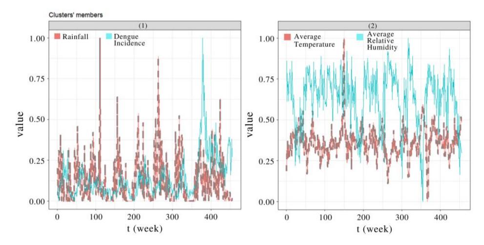
Figure 3 Results of K-Medoids Clustering in East Jakarta. Cluster 1 consisted of rainfall and Dengue incidence, and cluster 2 consisted of average temperature and relative humidity. In both clusters, the dashed line is the medoid.
For K-Medoids Clustering, we found that clustering the data into two clusters maximized the silhouette coefficient to 0.2782666. Clustering was performed on the normalized time-series data. The results of K-Medoids clustering are shown in Figure 3, in which the -axis represents time (week) and the -axis represents the data value at time . The medoid of each cluster is the time-series data point representing the cluster's other data points. Rainfall is the medoid of cluster 1; the average temperature is the medoid of cluster 2.
In cluster 1 we can see that high fluctuations in rainfall tended to be followed by an increase of Dengue incidence a few weeks later. For example, rainfall increased at around the 210th week, followed by an increase in Dengue incidence at the 219th week. Thus, the fluctuations of Dengue incidence had a similar pattern to that of rainfall occurring a few weeks earlier. However, there were periods when a high fluctuation in rainfall did not produce a corresponding increase in the incidence of Dengue. For example, when rainfall increased at around the 110th week, there was no spike in Dengue incidence. The lack of spike is due to loss of mosquito breeding grounds from excessive rainfall, which drift away the mosquito larvae and make them perish, as shown in previous studies [7,33]. In cluster 2, a drastic increase in the average temperature tended to be followed by a drastic decrease in average relative humidity in the next few weeks. For example, the average temperature increased at around the 150th week, followed by a decrease in average relative humidity at the 170th week.
With FCM Clustering, we found that clustering the data into three clusters maximized MPC to 0.6682991. Figure 4 illustrates our result. The centroid of each cluster in the form of a time series is the average of all time-series in that cluster.
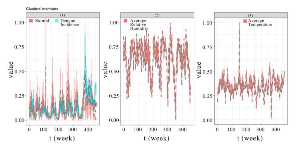
Figure 4 Results of FCM Clustering in East Jakarta. Cluster 1 consisted of rainfall and Dengue incidence, cluster 2 consisted of average relative humidity, and cluster 3 consisted of average temperature. In all clusters, the dashed line is the centroid.
For cluster 1, we again found that a high increase in rainfall tended to be followed by an increase in Dengue incidence a few weeks later. For example, rainfall increased at around the 160th week, followed by an increase in Dengue incidence at the 170th week. Both average relative humidity and temperature occupy cluster 2 and cluster 3, respectively, because they do not have a similar pattern.
3.1.2 Clustering Results for South Jakarta
For South Jakarta, we clustered six time-series variables, i.e. rainfall, Dengue incidence, average temperature, average relative humidity, average sunshine, and average wind speed. We again used the K-Medoids and FCM algorithms to cluster the data.
With K-Medoids Clustering, we found that using two clusters maximized the silhouette coefficient to 0.2828224. Clustering was performed on the time-series
data with the results shown in Figure 5. Average wind speed and average temperature were the medoids of cluster 1 and cluster 2, respectively.
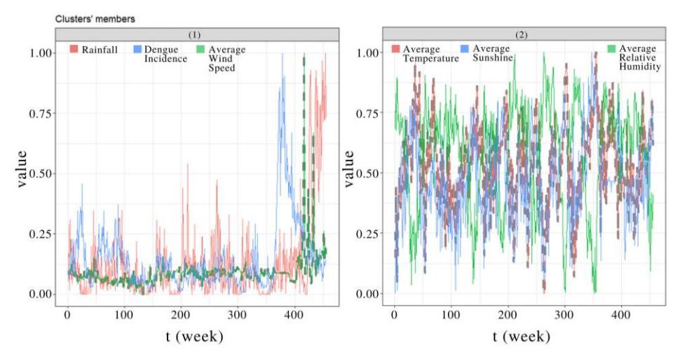
Figure 5 Results of K-Medoids Clustering in South Jakarta. Cluster 1 consisted of rainfall, Dengue incidence, and average wind speed, and cluster 2 consisted of average temperature, average sunshine, and average relative humidity. In both clusters, the dashed line is the medoid of each cluster.
As in the case of East Jakarta, we can see that an increase in rainfall was often followed by increased Dengue incidence a few weeks later. Thus, the fluctuations of Dengue incidence had a similar pattern to that of rainfall occurring a few weeks earlier. Based on the clustering results, we also found that the average temperature, average sunshine, and average relative humidity of South Jakarta all have similar patterns.
With FCM Clustering, we found that using two clusters maximized MPC to 0.48288. Figure 6 illustrates our result.
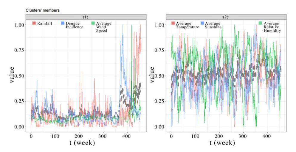
Figure 6 Results of FCM Clustering in South Jakarta. Cluster 1 consisted of rainfall, Dengue incidence, and average wind speed and cluster 2 consisted of time-series data on average temperature, average sunshine, and average relative humidity. In all the clusters, the dashed line is the centroid.
We can see that both algorithms obtained similar results. The only difference is that the medoids obtained from K-Medoids Clustering differ from the centroids from FCM Clustering. Subsection 4.1 contains a further explanation regarding the results for other regions in DKI Jakarta.
3.2 Implementation of K-Medoids and Fuzzy C-Means Clustering with Non-Time-Series Data
For non-time-series clustering, each of our data points was in the form of a tuple containing values of the variables taken in a specific region in a specific year. Each data point was labeled with the name of the region and year. For example, 'Year 2009: West Jakarta' means that the data point contained information on the variables for West Jakarta in 2009. The data consisted of 40 data points obtained from 2009 to 2016, where each year contains data from all five regions. Each data point contained information on average temperature, rainfall, average relative humidity, and Dengue incidence.
With K-Medoids Clustering, we found that using five clusters maximized the silhouette coefficient to 0.4. By running the program, we obtained the clustering results shown in Tables 1 and 2.
Cluster Medoid Average temperature (℃) Rainfall (mm) Average relative humidity (%) Dengue incidence 1 27.62267123 1674.120359 78.42917808 499 2 28.52520548 1632.5 74.26575342 336 3 27.57099446 2606.796583 80.6357834 1012 4 28.42219178 2289.4 77.25753425 468 5 27.79672131 3038.5 83.01912568 2975
Table 1 K-Medoids clustering results.
Table 2 Member list for each cluster obtained from K-medoids clustering.
| Cluster | Members | |
|---|---|---|
| 1 | Year 2009: East Jakarta, South Jakarta, West Jakarta | |
| Year 2011: East Jakarta, South Jakarta, West Jakarta | ||
| Year 2012: East Jakarta, South Jakarta, West Jakarta | ||
| Year 2015: East Jakarta, South Jakarta, West Jakarta | ||
| 2 | Year 2009: Central Jakarta, North Jakarta | |
| Year 2011: Central Jakarta, North Jakarta | ||
| Year 2012: Central Jakarta, North Jakarta | ||
| Year 2015: Central Jakarta, North Jakarta | ||
| 3 | Year 2010: East Jakarta, South Jakarta, West Jakarta | |
| Year 2013: East Jakarta, South Jakarta, West Jakarta | ||
| Year 2014: East Jakarta, South Jakarta, West Jakarta | ||
| Year 2016: East Jakarta | ||
| 4 | Year 2010: Central Jakarta, North Jakarta | |
| Year 2013: Central Jakarta, North Jakarta | ||
| Year 2014: Central Jakarta, North Jakarta | ||
| Year 2016: Central Jakarta, North Jakarta | ||
| 5 | Year 2016: South Jakarta, West Jakarta | |
Table 1 gives the medoid of each cluster by giving some values of the four variables, which can represent the information contained in that cluster, while Table 2 lists the members of each of the five clusters. For example, cluster 5 contains data points for South and West Jakarta in 2016.
Table 3 Fuzzy C-means clustering results.
| Centroid | |||||
|---|---|---|---|---|---|
| Cluster | Average temperature (℃) | Rainfall (mm) | Average relative humidity (%) | Dengue incidence | |
| 1 | 27.70050708 | 1670.212411 | 77.48549455 | 584.0761336 | |
| 2 | 27.7634214 | 2631.663034 | 80.80149982 | 2252.335648 | |
| 3 | 27.55105967 | 2727.798498 | 80.34074157 | 757.3704623 | |
| 4 | 28.41779432 | 2510.872042 | 76.9545875 | 559.2256772 | |
| 5 | 28.50786759 | 1623.470482 | 74.37180387 | 326.8854279 | |
With FCM Clustering, we found that using five clusters maximized the MPC to 0.4583934. We display the clustering results in Tables 3 and 4.
Table 4 Member list for each cluster obtained from fuzzy Cmeans clustering
| Cluster | Members | ||
|---|---|---|---|
| 1 | Year 2009: East Jakarta, South Jakarta, West Jakarta | ||
| Year 2011: East Jakarta, South Jakarta, West Jakarta | |||
| Year 2012: East Jakarta, South Jakarta, West Jakarta | |||
| Year 2015: East Jakarta, South Jakarta, West Jakarta | |||
| 2 | Year 2010: West Jakarta | ||
| Year 2016: East Jakarta, South Jakarta, West Jakarta | |||
| 3 | Year 2010: East Jakarta, South Jakarta | ||
| Year 2013: East Jakarta, South Jakarta, West Jakarta | |||
| Year 2014: East Jakarta, South Jakarta, West Jakarta | |||
| 4 | Year 2010: Central Jakarta, North Jakarta | ||
| Year 2013: Central Jakarta, North Jakarta | |||
| Year 2014: Central Jakarta, North Jakarta | |||
| Year 2016: Central Jakarta, North Jakarta | |||
| 5 | Year 2009: Central Jakarta, North Jakarta | ||
| Year 2011: Central Jakarta, North Jakarta | |||
| Year 2012: Central Jakarta, North Jakarta | |||
| Year 2015: Central Jakarta, North Jakarta | |||
Table 3 contains the centroid of each cluster obtained in Table 4. As an illustration, Central and North Jakarta in clusters 4 and 5 (in Table 4) tended to have higher average temperature values. In addition, both regions had less rainfall, less average relative humidity, and fewer Dengue incidents than the other clusters (see data in Table 3).
We note that the results from K-Medoids and FCM Clustering are very similar. Clusters 1, 2, and 4 of Table 2 have the same members as clusters 1, 5, and 4 respectively, of Table 4. Furthermore, these clusters also have a medoid (in Table 1) that is almost the same as the centroid (in Table 3). The other clusters in Table 2 and Table 4 have only minor differences. Further discussion regarding the combined results of both clustering methods is given in Subsection 4.2.
4 Discussion
This section presents a discussion of the preceding results obtained from the clustering of data between 2009 and 2016. Subsection 4.1 contains a discussion of the results of K-Medoids and FCM Clustering using time-series data. Meanwhile, Subsection 4.2 discusses the results of both clustering algorithms using non-time-series data.
4.1 Discussion on K-Medoids and Fuzzy C-Means Clustering in Time-Series Data
The full results for the five regions in DKI Jakarta are summarized in Table 5.
Regions Methods Cluster 1 Cluster 2 Cluster 3 East Jakarta K-Medoids R, DI AT, ARH - FCM R, DI ARH AT Central Jakarta K-Medoids R, DI, AWS AT, AS, ARH - FCM R, DI AT, AS, ARH, AWS - North Jakarta K-Medoids R, DI AT, AS, ARH, AWS - FCM R, DI AT, AS, ARH, AWS - South Jakarta K-Medoids R, DI, AWS AT, AS, ARH - FCM R, DI, AWS AT, AS, ARH - West Jakarta K-Medoids R, DI AT, AS, ARH, AWS - FCM R, DI, AWS AT, AS, RKR -
Table 5 Results of clustering of time-series data.
In Table 5, the symbol R denotes rainfall, AWS average wind speed, ARH average relative humidity, AS average sunshine, AT average temperature, and DI denotes Dengue incidence.
As an illustration, for the East Jakarta area, two clusters were produced using K-Medoids Clustering. Cluster 1 consisted of rainfall and Dengue incidence, and cluster 2 consisted of average temperature and relative humidity. FCM Clustering formed three clusters, with cluster 1 consisting of rainfall and Dengue incidence, cluster 2 consisting of average relative humidity, and cluster 3 consisting of average temperature.
From these results, we infer that rainfall and Dengue incidence were always clustered together. In addition, average sunshine, temperature, and relative humidity all occupy the same cluster (except for East Jakarta, where average sunshine was not considered as a variable). Thus, rainfall was the weather variable whose pattern most closely resembled Dengue incidence in DKI Jakarta. Therefore, rainfall can be used to estimate Dengue incidence. In addition, average temperature, relative humidity, and sunshine all have a different pattern from Dengue incidence. However, the three variables are not necessarily unrelated to Dengue incidence.
4.2 Discussion on K-Medoids and Fuzzy C-Means Clustering in Non-Time-Series Data
This subsection discusses the results obtained from Tables 1-4. Notable observations from the K-Medoids Clustering results are summarized in Table 6.
Note that the results from FCM Clustering in Tables 3 and 4 have a similar interpretation to Table 6. Dividing the same regions as in Table 6 yields similar results to those from Table 6. Based on Table 6, Dengue incidence tends to be positively correlated with both rainfall and average relative humidity. If rainfall and average relative humidity increase, Dengue incidence will also increase. In contrast, Dengue incidence and average temperature tend to be negatively correlated. These results are supported by the study of Tanawi, et al. [34], which was conducted using cross-correlation.
Table 6 Results of clustering with non-time-series data using K-medoids clustering.
| Parameters | Central and North Jakarta | East, South, and West Jakarta |
|---|---|---|
| Average Temperature | Tends to be higher. In Table 1, the highest average temperature (28.52520548 ℃) is in cluster 2. Cluster 2 contains the regions for the years 2009, 2011, 2012, and 2015 as shown in Table 2. | Tends to be lower. In Table 1, the lowest average temperature (27.62267123 ℃) is in cluster 1. In Table 2, cluster 1 contains the regions for 2009, 2011, 2012, and 2015. |
| Rainfall | Tends to be lower. In Table 1, the lowest rainfall (1632.5 mm) is in cluster 2. Cluster 2 in Table 2 contains the regions for the years 2009, 2011, 2012, and 2015. | Tends to be higher. For example, in Table 1, the higher rainfall (1674.12 mm) is in cluster 1. Cluster 1 in Table 2 contains the regions for the years 2009, 2011, 2012, and 2015. |
| Average Relative Humidity | Tends to be lower. The regions had similar average relative humidity between 2009 and 2016, that is around 75.71%. | Tends to be higher. The regions had similar average relative humidity between 2009 and 2016, that is around 80.12%. |
| Dengue Incidence | Tends to be lower. For example, from Table 1, cluster 2 experienced a lower Dengue incidence (336) relative to cluster 1 (499) in other regions in the same years in Table 2. | Tends to be higher. For example, cluster 1 in Table 1 has a higher Dengue incidence (499) compared to cluster 2. |
Based on these results, we can use weather variable data to predict the possibility of spikes in dengue incidence. Regions measuring values of rainfall and average relative humidity that show an increasing trend require more attention from the government, especially when entering the rainy season. Various health facilities need to be prepared to anticipate an increase in the number of Dengue patients.
5 Conclusions
In this research, by clustering time-series data using K-Medoids and Fuzzy C-Means Clustering, we found that rainfall had the most similar pattern to Dengue incidence in five regions of DKI Jakarta. Therefore, rainfall can be used to estimate of the occurrence of Dengue incidence. However, this is not the case with other weather factors, since average temperature, average relative humidity, and average sunshine do not have similar patterns to Dengue incidence.
In addition, with non-time-series clustering using K-Medoids and FCM Clustering, Dengue incidence, relative humidity, and the amount of rainfall tended to be positively correlated. Moreover, Dengue incidence and average temperature were negatively correlated.
This study especially showed that past weather data correlates with present Dengue incidence. Hence, prompt analysis of weather data should be given priority for combating potential dengue outbreaks.
Based on these results, the use of weather data to predict the possibility of spikes in dengue incidence should be more utilized. Regions with both rainfall and average relative humidity that shown an increasing trend, require more attention from the government, especially when entering the rainy season. Cooperation between the DKI Jakarta government and the community is necessary because Dengue can be prevented through activities suggested by the Health Office, including cleaning mosquito nests, closing water reservoirs, and burying used goods, so that they do not become mosquito breeding grounds.
There are several suggestions for future research, such as using other time-series clustering methods to classify time-series data, such as TADPole, k-Shape, and Fuzzy C-Medoids Clustering. In addition, further studies can also be conducted elsewhere in other regions in Indonesia, especially in areas with high Dengue incidence.
Acknowledgment
This research was funded by Universitas Indonesia, with the grant NKB-1997/UN2.RST/HKP.05.00/2020. Appreciation goes to BMKG Indonesia and the DKI Jakarta Health Department, whose generous cooperation made this research possible.