
1 Introduction
Cigarettes are among the most dangerous killers in the world. The content of chemical compounds in cigarettes can be bad for the health of smokers and also for people in their environment. The chemicals in cigarettes can trigger various diseases, such as heart failure, hypertension, lung cancer, etc. This is caused by approximately 4000 chemical compounds contained in cigarettes, of which at least 200 are poisonous and dangerous to health, while 43 other chemicals can provoke cancer. Inhaling cigarettes can cause coma or even death. The cigarette compound that is most often mentioned is nicotine. Possible effects of nicotine exposure are vomiting, convulsions, and stress on the central nervous system. Tar, another major compound found in cigarettes, is carcinogenic. Tar also increases the risk of diabetes, heart disease, and fertility problems. Another toxic compound that makes up cigarettes is hydrogen cyanide. The effects of this compound can weaken the lungs and cause fatigue, headaches, and nausea. Benzene is a residue from burning cigarettes that can damage white blood cells, reducing endurance and increasing the risk of leukemia. Another residue of burning cigarettes is formaldehyde. Formaldehyde increases the risk of nasopharyngeal cancer. Arsenic is a compound in cigarette smoke that is a firstclass carcinogen. A high level of arsenic exposure increases the risk of skin cancer, lung cancer, urinary tract cancer, kidney cancer, and liver cancer. As for cadmium, about 40-60 percent of the cadmium found in cigarette smoke is absorbed into the lungs when smoking. High levels of cadmium in the body can cause sensory disorders, vomiting, diarrhea, seizures, muscle cramps, kidney failure, and cancer. One last dangerous compound found in cigarettes is ammonia. Ammonia is a colorless poisonous gas with a strong smell. The cigarette industry uses ammonia to boost the effects of nicotine addiction. Longterm impacts are pneumonia and throat cancer.
The above description of the chemical substances contained in cigarettes shows the danger of smoking, but public awareness about the related health risks is insufficient and in Indonesia smoking is still commonplace. Some children in Indonesia start smoking as early as at the age of 9. The age of smoking the first cigarette is generally well before the age of 18, ranging from 11-13 years. There are some factors that stimulate addiction. Biologically, the nicotine contained in cigarettes can suppress the brain's ability to gain pleasure from cigarettes, so that smokers always need higher levels of nicotine to achieve the same level of satisfaction, causing dependency on cigarettes.
Phenomena in the real world and their dynamics can be studied by using mathematical modeling, i.e., converting real-world phenomena into mathematical formulations. Several studies on smoking with a mathematical approach have been reported [1-6]. The results can be used for example to inform policymaking. Many mathematical models on smoking have been built based on the assumptions of the researchers. In [7], the used mathematical model was divided into four sub-classes, namely potential smokers, individuals who smoke < 20 cigarettes per day, heavy smokers who smoke > 20 cigarettes per day, and people who have stopped smoking. Control was carried out using two optimal controls, namely anti-smoking campaign and media campaign. Sikander et al. [8] used the mathematical model that was developed in [9]. Another smoking mathematical model is presented in [10], where the population is divided into five sub-classes, namely potential smokers, occasional smokers, active smokers, smokers who have temporarily stopped smoking, and smokers who have stopped permanently. In the present study, a mathematical model based on [10] was used. The main contribution of this study lies in providing four controls with the ultimate aim of reducing the population of individuals who smoke and increase the population of individuals who permanently stop smoking.
The rest of this paper is organized as follows. Section 2 explains the dynamic model of smoking used in this study. Section 3 is about the formulations, the existence of optimal controls and their solution. The simulation results and discussion are presented in Section 4. The last section provides the conclusion of this research.
2 Dynamic Model of Smoking
In this section, the mathematical model used in this study is discussed. () is the total population at time , divided into five subclasses, i.e., () is the population of potential smokers, () is the population of occasional smokers, () is the population of active smokers, () is the population of individuals who have temporarily stopped smoking, and () is the population of individuals who have stopped smoking permanently. The mathematical representation of the smoking dynamic model is as follows [10]:
\[\frac{dP}{dt} = \Lambda - \beta P(t)S(t) - \mu P(t)\] \[\frac{dO}{dt} = \beta P(t)S(t) - \alpha_1 O(t) - \mu O(t)\] \[\frac{dS}{dt} = \alpha_1 O(t) + \alpha_2 S(t)Q_t(t) - (\mu + \gamma)S(t)\] \[\frac{dQ_t}{dt} = -\alpha_2 S(t)Q_t(t) - \mu Q_t(t) + \gamma (1 - \sigma)S(t)\] \[\frac{dQ_P}{dt} = \sigma \gamma S(t) - \mu Q_P(t)\] (1)
This model can be represented in graphic form as in Figure 1.
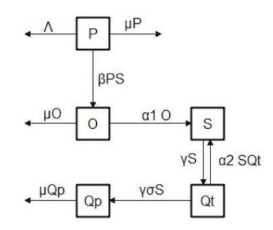
Figure 1 Compartmental diagram.
This dynamic model of smoking was employed with optimal control, consisting of government prohibition of the utilization of smoking in public spaces, antismoking gum, anti-nicotine drug, and anti-smoking education campaign. The goals are to minimize the cost function of reducing the number of people who smoke and increasing the number of individuals who stop smoking permanently.
3 Optimal Control
3.1 Optimal Control Formulations
This section discusses a strategy of optimal control that is suitable for the dynamics of model in Eq. (1). A classical control system design, generally speaking, is a process of trial and error to determine an 'acceptable' or 'admissible' system design. Modern technology is needed for complex systems and multi-input/multi-output (MIMO) systems. For this reason, a new approach using optimal control theory has been developed [11,12]. Optimal control theory was first developed in the 1950s. There are two methods to solve optimal control problems, namely dynamic programming, introduced in [13], and the PMP method, introduced in [14].
The goal of optimal control is to determine the optimal input while satisfying the physical constraints by minimizing or maximizing some performance criteria. In simple terms, the control has to bring the system from the state at time 0, (0 ), to the final state at terminal time , () in such a way that it produces a result in terms of the maximum or minimum value of the defined objective function.
Four controls were considered in this study. The controls were constructed in Eq. (1), by combining them into the standard model, which can be represented as follows:
\[\frac{dP}{dt} = \Lambda - \beta P(t)S(t) - (\mu + u_1 + u_4) P(t) \frac{dO}{dt} = \beta P(t)S(t) - (\alpha_1 + \mu + u_2 + u_4)O(t) \frac{dS}{dt} = \alpha_1 O(t) + \alpha_2 S(t)Q_t(t) - (\mu + \gamma + u_3 + u_4)S(t) \frac{dQ_t}{dt} = -\alpha_2 S(t)Q_t(t) - (\mu + u_2 + u_4)Q_t(t) + \gamma(1 - \sigma)S(t) \frac{dQ_P}{dt} = \sigma \gamma S(t) - \mu Q_P(t) + (u_1 + u_4)P(t) + (u_2 + u_4)O(t) + (u_3 + u_4)S(t) + (u_2 + u_4)Q_t(t)\] (2)
Providing suitable controls can reduce the number of individuals who smoke and the number of potential smokers to lower levels. Conversely, if the four controls are not given, the number of individual smokers and potential smokers will increase and the number of individuals who stop smoking will decrease. In establishing the objective function, we considered the control problems in Eq. (2). The following objective function was obtained:
\[J(u(t)) = \int_0^{t_f} \left( S(t) - Q_P(t) + \frac{1}{2} \left( k_1 u_1^2(t) + k_2 u_2^2(t) + k_3 u_3^2(t) + k_4 u_4^2(t) \right) \right) dt\] (3)
The aim of this study was to minimize J(u(t)) subject to its constraints by using the optimal control method.
3.2 Optimal Control Existence
The methodology was used to demonstrate the presence of ideal control to be applied to the model [15-16]. It was assumed that the control system in Eq. (2) can be rewritten as follows:
\[\zeta_t = C\zeta + F(\zeta) \tag{4}\] where the vector of the state variables is
\[\zeta = [P(t), O(t), S(t), Q_t(t), Q_P(t)]^T\] and
\[C = \begin{pmatrix} -a & 0 & 0 & 0 & 0 \\ 0 & -b & 0 & 0 & 0 \\ 0 & \alpha_1 & -c & 0 & 0 \\ 0 & 0 & d & -e & 0 \\ f & a & h & m & -u \end{pmatrix}\] where,
\[a = (\mu + u_1 + u + 4)\] \[b = (\alpha_1 + \mu + u_2 + u_4)\] \[c = (\mu \gamma + u_3 + u_4)\] \[d = \gamma (1 - \sigma)\] \[e = (\mu + u_2 + u_4)\] \[f = u_1 + u_4\] \[g = u_2 + u_4\] \[h = \sigma \gamma + u_3 + u_4\] \[i = u_2 + u_4\] \[F(\zeta) = (\Lambda - \beta PS \beta PS \alpha_2 SQ_t - \alpha_2 SQ_t 0)\]
Eq. (4) is a nonlinear differential equation with bounded coefficients, where \(\zeta_t\) is the time derivative of \(\zeta\). We have:
\[B(\zeta) = C(\zeta) + F(\zeta)\]
\[\begin{split} F(\zeta_1) - F(\zeta_2) &= \left( -\beta P_1 S_1 + \beta P_2 S_2 + \beta P_3 S_3 + \beta P_4 S_4 \, \beta P_1 S_1 - \right. \\ & \beta P_2 S_2 - \beta P_3 S_3 - \beta P_4 S_4 \, \alpha_2 S_1 Q_{t_1} - \alpha_2 S_2 Q_{t_2} - \\ & \alpha_2 S_3 Q_{t_3} - \alpha_2 S_4 Q_{t_4} - \alpha_2 S_1 Q_{t_1} + \alpha_2 S_2 Q_{t_2} + \\ & \alpha_2 S_3 Q_{t_3} + \alpha_2 S_4 Q_{t_4} \, 0 \, \right) \end{split}\]
Therefore,
\[\text{[rumus tidak dapat ditampilkan dengan baik — lihat PDF asli]}\]
We have \(|B(\zeta_1) - B(\zeta_2) \le Z|\zeta_1 - \zeta_2|\), where \(Z = max\{(2\beta + 2\alpha_2)\Lambda/\mu, |C|\} < \infty\). It can be seen that \(B(\zeta)\) is uniformly Lipschitz continuous, so that by looking at the definition of \(u_i\) it can be concluded that a solution of the controlled system (4.1) exists.
3.3 Optimal Control Solutions
Let optimal control Eqs. (2)-(3) be written with a Hamiltonian function as follows:
\[H = L + \sum_{j=1}^{5} \lambda_j(t)g_j \tag{5}\] where the Lagrangian function can be written as:
\[L(S, Q_t, u_i) = A_1 S(t) - A_2 Q_P(t) + \frac{1}{2} [k_1 u_1^2(t) + k_2 u_2^2(t) + k_3 u_3^2(t) + k_4 u_4^2(t)]\] (6)
and
\[g_1 = \frac{dP}{dt}, g_2 = \frac{dO}{dt}, g_3 = \frac{dS}{dt}, g_4 = \frac{dQ_t}{dt}, g_5 = \frac{dQ_P}{dt}\] (7)
Thus, the following Hamiltonian function is obtained:
\[\begin{split} H &= \left( S(t) - Q_P(t) + \frac{1}{2} \left( k_1 u_1^2(t) + k_2 u_2^2(t) + k_3 u_3^2(t) + k_4 u_4^2(t) \right) + \\ &\quad \lambda_1 \left( \Lambda - \beta P(t) S(t) - \mu P(t) \right) + \lambda_2 (\beta P(t) S(t) - \alpha_1 O(t) - \\ &\quad \mu O(t) \right) + \lambda_3 \left( \alpha_1 O(t) + \alpha_2 S(t) Q_t(t) - (\mu + \gamma) S(t) \right) + \\ &\quad \lambda_4 \left( -\alpha_2 S(t) Q_t(t) - \mu Q_t(t) + \gamma (1 - \sigma) S(t) + \lambda_5 \sigma \gamma S(t) - \\ &\quad \mu Q_P(t) \right) \right) \end{split}\]
The PMP method was used to obtain the adjoint variables [17-23].
Theorem Given the solutions \(P^*(t)\), \(O^*(t)\), \(S^*(t)\), \(Q_t^*(t)\), \(Q_P^*(t)\) and the optimal controls \(u_1^*(t)\), \(u_2^*(t)\), \(u_3^*(t)\), \(u_4^*(t)\) of the appropriate condition system in Eqs. (2)-(4) are adjoint variables that satisfy the following equations:
\[\dot{\lambda}_{1} = -\left(\lambda_{1}\left(-\beta S - (\mu + u_{1} + u_{4})\right) + \lambda_{2}(\beta S) + \lambda_{5}(u_{1} + u_{4})\right) \dot{\lambda}_{2} = -\left(\lambda_{2}(\alpha_{1} + \mu + u_{2} + u_{4}) + \lambda_{3}\alpha_{1} + \lambda_{5}(u_{2} + u_{4})\right) \dot{\lambda}_{3} = -1 + \lambda_{1}(\beta P) + \lambda_{2}(\beta P) + \lambda_{3}\left(\alpha_{2}Q_{t} - (\mu + \gamma + u_{3} + u_{4})\right) + \lambda_{4}\alpha_{2}Q_{t} + (\gamma(1 - \sigma)) + \lambda_{5}(\sigma\gamma + (u_{3} + u_{4})) \dot{\lambda}_{4} = -\lambda_{3}(\alpha_{2}S) + \lambda_{4}\left(-\alpha_{2}S - (\mu + u_{2} + u_{4})\right) + \lambda_{5}(u_{2} + u_{4}) \dot{\lambda}_{5} = -(-1 - \lambda_{5}\mu) \lambda_{i}(t_{f}) = 0, i = 1,2,3,4,5.\] (9)
\[u_1^*(t) = \min\left(\max\left(0, \frac{\lambda_1(t)P(t) - \lambda_5(t)P(t)}{k_1}\right), 1\right)\] (10)
\[u_{2}^{*}(t) = min\left(max\left(0, \frac{\lambda_{2}(t)o(t) + \lambda_{4}(t)Q_{t}(t) - \lambda_{5}(t)\left(o(t) + Q_{t}(t)\right)}{k_{2}}\right), 1\right)\](11)
\[u_3^*(t) = \min\left(\max\left(0, \frac{\lambda_3(t)S(t) - \lambda_5(t)S(t)}{k_3}\right), 1\right)\] (12)
\[u_4^*(t) = \min\left(\max\left(0, \frac{A}{k_4}\right), 1\right) \tag{13}\] where,
\[A = \lambda_1(t)P(t) + \lambda_2(t)O(t) + \lambda_3(t)S(t) + \lambda_4(t)Q_t(t) - \lambda_5(t)(P(t) + O(t) + S(t) + Q_t(t)\]
Proof: Distinguish the Hamiltonian equation H by its respective conditions and use the PMP method to obtain the equations of the adjoint variables.
\[\lambda_1(t) = -\frac{\partial H(t)}{\partial P}\]
\[\lambda_{1}\dot{}(t) = -\frac{\partial H(t)}{\partial O}\] \[\lambda_{3}\dot{}(t) = -\frac{\partial H(t)}{\partial S}\] \[\lambda_{4}\dot{}(t) = -\frac{\partial H(t)}{\partial Q_{t}}\] \[\lambda_{5}\dot{}(t) = -\frac{\partial H(t)}{\partial Q_{P}}\]
We use the optimal conditions and obtain the following equations:
\[\begin{split} \frac{\partial H}{\partial u_1} &= k_1 u_1^*(t) - \lambda_1(t) P(t) + \lambda_5(t) P(t) = 0, at \ u_1 = u_1^*(t) \\ \frac{\partial H}{\partial u_2} &= k_2 u_2^*(t) - \lambda_2(t) O(t) - \lambda_4(t) Q_t(t) + \lambda_5(t) \big( O(t) + Q_t(t) \big) 0, \\ \text{at } u_2 &= u_2^*(t) \\ \frac{\partial H}{\partial u_3} &= k_3 u_3^*(t) - \lambda_3(t) S(t) + \lambda_5(t) S(t) = 0, at \ u_3 = u_3^*(t) \\ \frac{\partial H}{\partial u_4} &= k_4 u_4^*(t) - \lambda_1(t) P(t) - \lambda_2(t) O(t) + \lambda_3(t) S(t) - \lambda_4(t) Q_t(t) + \lambda_5(t) \big( P(t) + O(t) + S(t) + Q_t(t) \big) = 0, \ at \ u_4 = u_4^*(t) \end{split}\]
Then we obtain:
\[\begin{split} u_{1}^{*}(t) &= min\left(max\left(0, \frac{\lambda_{1}(t)P^{*}(t) - \lambda_{5}(t)P^{*}(t)}{k_{1}}\right), 1\right) \\ u_{2}^{*}(t) &= min\left(max\left(0, \frac{\lambda_{2}(t)O^{*}(t) + \lambda_{4}(t)Q_{t}^{*}(t) - \lambda_{5}(t)\left(O^{*}(t) + Q_{t}^{*}(t)\right)}{k_{2}}\right), 1\right) \\ u_{3}^{*}(t) &= min\left(max\left(0, \frac{\lambda_{3}(t)S^{*}(t) - \lambda_{5}(t)S^{*}(t)}{k_{3}}\right), 1\right) \\ u_{4}^{*}(t) &= min\left(max\left(0, \frac{\lambda_{1}(t)P^{*}(t) + \lambda_{2}(t)O^{*}(t) + \lambda_{3}(t)S^{*}(t) + \lambda_{4}(t)Q_{t}^{*}(t)}{k_{4}}\right), 1\right) \end{split}\]
Thus, we obtain the following optimal control function:
\[\text{[rumus tidak dapat ditampilkan dengan baik — lihat PDF asli]}\] where,
\[q = \frac{\lambda_2(t)O^*(t) + \lambda_4(t)Q_t^*(t) - \lambda_5(t)(O^*(t) + Q_t^*(t))}{k_2}\] \[r = \frac{\lambda_1(t)P^*(t) + \lambda_2(t)O^*(t) + \lambda_3(t)S^*(t) + \lambda_4(t)Q_t^*(t)}{k_4}\]
The optimal control system is given by:
\[\begin{split} &\frac{dP^*(t)}{dt}, \frac{do^*(t)}{dt}, \frac{dS^*(t)}{dt}, \frac{dQ_t^*(t)}{dt}, \frac{dQ_P^*(t)}{dt} \\ &\dot{\lambda}_1 = -\left(\lambda_1 \left(-\beta S - (\mu + u_1 + u_4)\right) + \lambda_2 (\beta S) + \lambda_5 (u_1 + u_4)\right) \\ &\dot{\lambda}_2 = -\left(\lambda_2 (\alpha_1 + \mu + u_2 + u_4) + \lambda_3 \alpha_1 + \lambda_5 (u_2 + u_4)\right) \\ &\dot{\lambda}_3 = -(1 + \lambda_1 (\beta P) + \lambda_2 (\beta P) + \lambda_3 \left(\alpha_2 Q_t - (\mu + \gamma + u_3 + u_4)\right) + \lambda_4 (\alpha_2 Q_t + (\gamma (1 - \sigma)) + \lambda_5 (\sigma \gamma + (u_3 + u_4))) \\ &\dot{\lambda}_4 = -\left(\lambda_3 (\alpha_2 S) + \lambda_4 \left(-\alpha_2 S - (\mu + u_2 + u_4)\right) + \lambda_5 (u_2 + u_4)\right) \\ &\dot{\lambda}_5 = -(-1 - \lambda_5 \mu) \\ &u_1^*(t) = \min\left(\max\left(0, \frac{\lambda_1 (t) P(t) - \lambda_5 (t) P(t)}{k_1}\right), 1\right) \\ &u_2^*(t) = \min\left(\max\left(0, \frac{\lambda_2 (t) O(t) + \lambda_4 (t) Q_t (t) - \lambda_5 (t) (O(t) + Q_t (t))}{k_2}\right), 1\right) \\ &u_3^*(t) = \min\left(\max\left(0, \frac{\lambda_3 (t) S(t) - \lambda_5 (t) S(t)}{k_3}\right), 1\right) \\ &u_4^*(t) = \min\left(\max\left(0, \frac{A_4 (t) B(t) - \lambda_5 (t) S(t)}{k_4}\right), 1\right) \end{split}\]
Thus, it is easy to see that the theorem has been proven.
4 Results and Discussion
In this section, we use a numerical method to solve the optimal control problem [24-27]. In this study we used the PMP method by employing the fourth-order Runge-Kutta. The parameter values are presented in Table 1.
Figure 2 shows the numerical solution of the smoking problem with initial conditions P(0) = 40, O(t) = 10, S(t) = 20, \(Q_t(t) = 10\), \(Q_P(t) = 5\). It shows the dynamic behavior of the smoking model without control. From this figure it can be seen that the population of potential smokers decreased drastically in the beginning but then gradually increased. The number of occasional smokers increased, the number of active smokers decreased, while the number of smokers who temporarily stop smoking also decreased. Lastly, the number of individuals who permanently stop smoking showed an increase.
| Parameters | Values | Descriptions |
|---|---|---|
| 𝛬 | 1 | Recruitment rate in 𝑃(𝑡) |
| 𝜇 | 0.001 | Natural death rate |
| 𝛽 | 0.14 | Effective contact rate between 𝑆(𝑡) and 𝑃(𝑡) |
| 𝛼1 | 0.002 | Rate at which occasional smokers become regular smokers |
| 𝛼2 | 0.0025 | Contact rate among smokers and people who stop smoking but return to smoking |
| 𝛾 | 0.8 | Rate of people who stop smoking |
| 𝜎 | 0.1 | Rate of people who stop smoking permanently |
Table 1 Parameter value and descriptions.
The treatment with an anti-nicotine drug for 25 days was considered here, since long-term treatment with drugs has the potential to have dangerous side effects and the best time for vaccination is probably in the early stages of a disease. The non-smoking population who can potentially become smokers is shown in Figure 3(a). This population showed a significant decrease on the first day. For the following day the graph shows an increase but not a significant one. After giving control, the number of potential smokers on the 20th day increased slightly compared to before introducing the control. This shows that this population is likely to continue decreasing if it is given this control for a longer period of time.
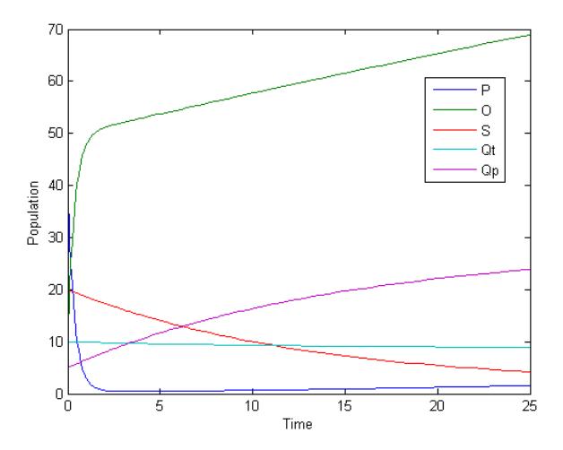
Figure 2 Plot of the model without control.
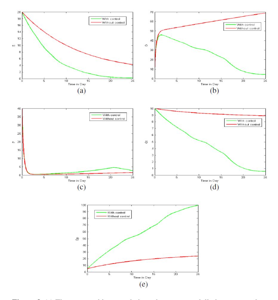
Figure 3 (a) The non-smoking population who can potentially become smokers with and without control. (b) The population of individuals who smokes occasionally with and without control. (c) The population of individuals who actively smoke with and without control. (d) The population of individuals who temporarily stopped smoking with and without control. (e) The population of individuals who have stopped smoking permanently with and without control.
For the population who smokes occasionally, control was given in the form of anti-smoking gum and government prohibition of smoking in public spaces. In Figure 3(b) it can be seen that on the first day a significant increase occurred and on the following days it further increased. After being given the control, the population who smoke occasionally showed a significant increase on the first day but a decrease on the following days. In contrast to before control, on the first day this population also showed an increase but not as large as before control. After that, the control started to show an effect.
Figure 3(c) shows the population of individuals who actively smoke with and without control. The control suggested for this population is anti-nicotine drug treatment and government prohibition of smoking in public spaces. The performed simulations showed that the population of active smokers decreased from the first day to the end of the simulation. The population with control also showed a decrease, but more significantly than before being given the controls. Thus, the controls had a good result in this case.
The population of individuals who temporarily stopped smoking is presented in Figure 3(d). The red line describes the simulation results without control and the green line shows the simulation results with control. For this population, the control given was in the form of anti-smoking gum and government prohibition of smoking in public spaces. Without control, the simulation results showed a decrease of this population from the first day to the 25th day, but with control this population decreased exponentially.
This study recommends providing controls in the form of anti-smoking education campaign, anti-smoking gum, anti-nicotine drug, and government prohibition of smoking in public spaces to the population of individuals who have stopped smoking permanently, see Figure 3(e). The simulation results show that from the beginning to the end of the simulation period there was an increase of the number of individuals who stopped smoking permanently. After giving control, there was a more significant increase. Giving control to this population gave better results compared to without control. Thus, this strategy shows the effectiveness of giving control.
5 Conclusion
A mathematical model of smoking was presented by considering four control variables, namely anti-smoking education campaign, \(u_1(t)\); anti-smoking gum, \(u_2(t)\); anti-nicotine drug treatment, \(u_3(t)\); and government prohibition of smoking in public spaces, \(u_4(t)\). The aim of the control was to reduce the population of individuals who smoke and increase the population of individuals who permanently stop smoking. The existence of optimal control in the mathematical model of smoking dynamics was proven. In this study, we find that the PMP method gives the optimal control solution for the fourth-order Runge-Kutta as the numerical method. According to the obtained simulation results, it can be concluded that the control variables that were used have an impact in accordance with the desired purposes.