
1 Introduction
Officially named COVID-19, the novel coronavirus pneumonia outbreak was first identified in Wuhan, China in late December 2019. It is recognized as a severe respiratory illness similar to MERS-CoV and SARS-CoV. A review published on March 2, 2019 foresaw future SARS- or MERS-like coronavirus diseases in humans originating from bats, most likely in China [1].
Soon the COVID-19 outbreak was characterized as a pandemic and the World Health Organization (WHO) declared it a Public Health Emergency of International Concern on 30 January 2020. As of April 8, 2020, over 1,436,833 cases of COVID-19 had been reported to WHO, from over 209 countries and territories around the world with more than 82,421 fatalities and about 303,721 recoveries.
Obtaining epidemiological characteristics such as basic reproduction number, incubation period, infectious period, and death rate are crucial in better understanding the pandemic outbreak. Shortly after the first statistics were made available, various research studies of COVID-19 were carried out to estimate these parameter values, see e.g. [2,3]. A study [4] from January 2020 estimated the basic reproduction number 0 to range from 2.24 (95%CI: 1.96-2.55) to 5.71 (95%CI: 4.24-7.54) using the formula 0 = 1/(−), where M is the moment generating function for the serial interval of the COVID-19 and γ is the intrinsic growth rate. Another early work [5] estimated 0 to be 3.11 (95%CI, 2.39-4.13) using the deterministic SEIR metapopulation model. The same work estimated the transmission rate, , to be 1.94 (95%CI, 1.25-6.71) and the infectious period to be 1.61 days (95%CI, 0.35-3.23) in Wuhan, China. A review of twelve recent works showed that 0 ranges from 1.4 to 6.49, with a mean of 3.28, a median of 2.79 and an interquartile range (IQR) of 1.16 [6]. While early reports of the Chinese Center for Disease Control and Prevention [7] suggested the infectious period to be 9 days, another recent work [8] reported the mean infectious period to be 10.91 days (SD = 3.95).
For various mathematical models that have been formulated to forecast the development of the disease and estimating the parameters, we refer to [9] and references therein.
Our goal in this study was to estimate death rates for COVID-19 for selected representative countries. These parameter values were used to estimate the recovery rate and the basic reproduction number from a deterministic mathematical model. We then compared these results to see if there were any significant differences among countries.
The rest of the paper is organized as follows. First, we introduce the methodology, including data, the mathematical model, and the parameter estimation technique. Then comes the results section, where we report our findings. Finally, we end with a discussion section, where we interpret the findings and provide recommendations for future research.
2 Method
2.1 Data Set
This study used Johns Hopkins University's COVID-19 data made available via a GitHub repository [10]. The dataset includes confirmed, recovered, and death cases for almost all countries in the world over the period of January 22, 2019 to March 23, 2020 on a daily basis. The epidemiological characteristics of
COVID-19 in the USA, South Korea, Italy, France, China, and Iran were studied; this list of selected countries was based on cluster analysis.
2.2 Theoretical Model
Let N be the total population of a country. The following diagram summarizes the disease transmission process.
Figure 1 SIR model diagram.
The corresponding classical deterministic SIR epidemic model is given by
\[\frac{dS}{dt} = -\beta SI/N\] \[\frac{dI}{dt} = \beta SI/N - (\gamma + \mu)I\] \[\frac{dR}{dt} = \gamma R\] where, S, I, R are susceptible, infectious, and recovered classes and parameters β, γ, μ are transmission, recovery, and death rates, respectively. Since we had a dataset containing data recorded on a daily basis, we fixed our time units in terms of days. For this model, the basic reproduction number is given by the formula
\[R_0 = \frac{\beta}{\gamma + \mu} \tag{1}\]
We note that this is a system of autonomous nonlinear ordinary differential equations. The nonlinearity term SI is due to the law of mass-action, which is the reason for the absence of a non-trivial closed form. However, computer assisted numerical approximations are available. There are variations of this model, where one may include new classes, such as exposed and quarantine cases, or demographic characteristics such as birth rate, natural death rate, etc. As our parameter estimations fit well to the current model, we decided to use it as is.
2.3 Clustering
Before applying the statistics model (least square) and SIR method, this study verified the cluster analysis. As reported above, there are over 184 countries where a COVID-19 outbreak has occurred so far. Analyzing each country
separately and reporting results in a research article is not very convenient. Therefore, we decided to run cluster analysis to first group the countries according to similarity of confirmed cases and then select one representative country from each cluster. Here, cluster analysis was carried using country recovery rates (γ) and the country doubling periods of confirmed cases. The last equation of the SIR model is / = , which can be rewritten in discretized form as
\[\Delta R_t = R(t+1) - R(t) = \gamma I(t). \tag{2}\]
Both and () can be computed from the dataset and γ can be obtained as the slope of the equation. Before the confirmed case gets very large, one can safely assume that ≈ , which together with the second equation of SIR gives / = , with growth rate = − − . This has a solution () = (0) from which one can obtain
\[k = \frac{\log(I(t)) - \log(I(0))}{t},\] where time t was taken to be the last day available in the dataset and = 0 was taken so that (0) is nonzero. We note here that () in the model is the total number of infectious cases at time t, which is different from the total number of confirmed cases at time t. However, if I has exponential growth, then so does the total confirmed cases. Once the growth rate is estimated for each country, the doubling period is computed to be (ln 2)/.
We conducted k-means cluster analysis, which is sensitive to outliers. Hence, we first cleared outliers from our data using box plot analysis and then used the elbow method to determine the number of centroids. Finally, cluster analysis was carried out for the normalized variables, -scores, and one representative was selected from each cluster. Moreover, we did not completely avoid outliers; instead, we selected one representative country with a low doubling period and a very low recovery period.
2.4 Parameter Estimation
To estimate the parameters β, γ, μ for the SIR system one usually considers nonlinear least square analysis. However, models are simplified versions of real life systems and not always behave well with parameter estimations. What we did was estimate parameter γ using simple linear regression. Then, we used this point estimate in the SIR model to estimate β and μ. More specifically, we used the scipy.integrate.ode function in the Python programming language to simulate (), (), and (), with the following initial values: (0) = country population, (0) = the first observed number of cases in the country, and (0) = 0. Then, we called the scipy.optimize.curve_fit function for least-square
fitting of the theoretical model solution to the observed daily number of confirmed cases and recovered individuals. More specifically, we let \(I_0(t)\); \(R_0(t)\) be the observed confirmed cases and total recovered individuals at time moment t, respectively. Also, we let \(I_p(t; \beta; \mu; \gamma)\); \(R_p(t; \beta; \mu; \gamma)\) be the predicted/simulated confirmed cases and total recovered individuals at time moment t obtained from the SIR model using Python's scipy.integrate.ode function, given parameter values \(\beta\); \(\mu\); \(\gamma\). Consider the error function
\[\begin{split} Error(\beta;\mu;\gamma) &= \sum_{t=0}^{n} [I_o(t) - I_p(t;\beta;\mu;\gamma)]^2 + \left[R_o(t) - R_p(t;\beta;\mu;\gamma)\right]^2, \end{split}\] where n is the total number of days from the day when the first infected case occurred in a country to March 23, 2020. Then, given \(\gamma\) from the linear regression, the scipy:optimize:curve_fit function searches for positive numbers \(\beta\) and \(\mu\) to minimize the error function.
3 Results and Discussion
Table 1 Countries in Each Cluster
| Cluster | Number | Countries | |||
|---|---|---|---|---|---|
| 1 | 14 | Afghanistan, Australia, Cruise Ship, Egypt, Georgia, India, Japan, South Korea, Malaysia, Monaco, Nigeria, Russia, Singapore, United Arab Emirates | |||
| 2 | 25 | Albania, Armenia, Bangladesh, Brunei, Bulgaria, Chile, Colombia, Costa Rica, Cote d'Ivoire, Croatia, Cyprus, Germany, Greece, Israel, Lebanon, Luxembourg, Morocco, Poland, San Marino, Saudi Arabia, Slovakia, Switzerland, Trinidad and Tobago, Ukraine, US | |||
| 3 | 10 | Azerbaijan, Belgium, Burkina Faso, Iceland, Indonesia, Italy, Jamaica, Kuwait, Senegal, Spain | |||
| 4 | 5 | Belarus, France, Hungary, Iraq, Pakistan | |||
The countries with fewer data resulted in unrealistic doubling periods (over 10) and/or almost zero recovery rates (less than 0.0001), these countries were eliminated. Eliminating countries with a doubling period more than 10 resulted in 152 countries left. On the other hand, when we eliminated countries with a very small (< 0.0001) recovery rate, we were left with only 67 countries. The eliminated countries were those with few data reports or with missing data for recovered individuals. Further remaining outliers were cleared using box plot analysis, which resulted in 54 countries left. The final box plot results for the 54 countries are shown in Figure 2.
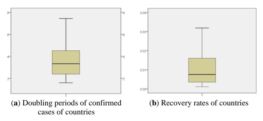
Figure 2 Box plots of recovery rates and cases doubling periods.
In Figure 3, the distributions of both doubling periods and recovery rates are shown. In particular, it can be seen that the mean doubling period for 54 countries was 3.60 (95%CI: 3.22-3.99).
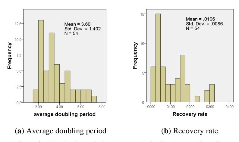
Figure 3 Distribution of doubling periods for the confirmed cases and recovery rates.
An elbow method summary is shown in Figure 4. Here we see that there are five points with sum of squared distances more than 1, suggesting to consider 5 clusters. However, with 5 clusters, some of the clusters would contain very few countries, and since the total remaining countries was only 54, we decided to set the number of clusters to 4.
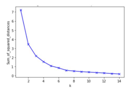
Figure 4 Scree plot for optimal k.
The bar charts of the -scores of the variables for each cluster are shown in Figure 5 and the list of countries in each cluster is given in Table 1. Both recovery rate and doubling period were found to be significant predictors, with F(3,50) = 76.19, p < 0.001 and F(3,50) = 45.17, p < 0.001 respectively.
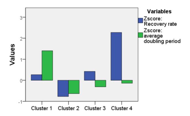
Figure 5 Scree plot for optimal k.
We see that the first cluster contained 14 countries with a high doubling period, the second cluster contained 25 countries with a low recovery rate and a low doubling period, the third contained 10 countries with a somewhat average recovery rate and an average doubling period, and the last cluster contained 5 countries with a high recovery rate.
We selected one representative country, i.e., Japan, Germany, Italy, and France from each cluster. We selected one more country as a representative of the outliers, namely the Netherlands, which had a low case doubling period (2.08 days) as well as a low recovery period (< 0.001).
For the selected countries, least square parameter estimation using the theoretical SIR model was carried out. The results are summarized in Table 2.
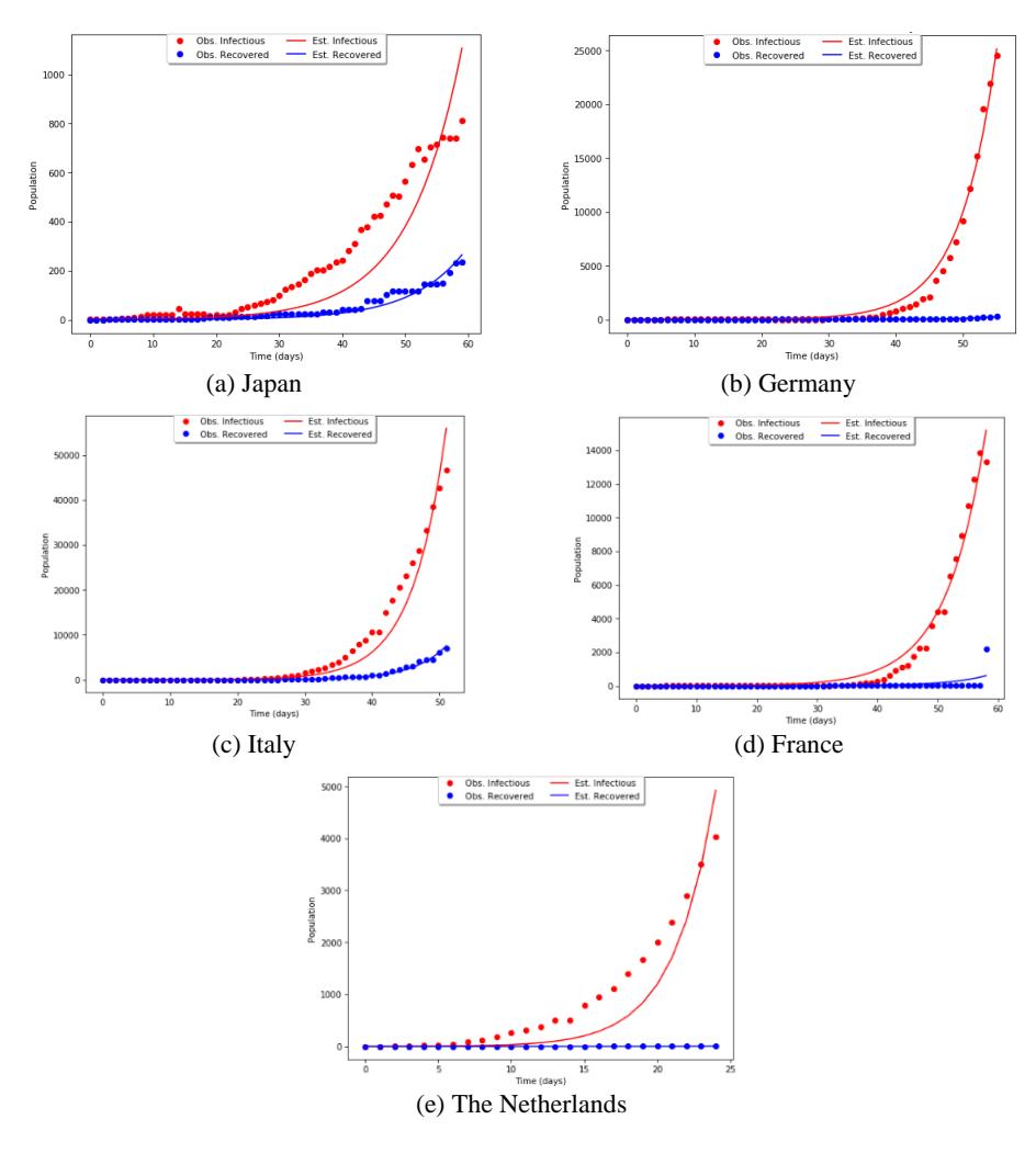
Figure 6 Plot of the data (dotted curve) vs. SIR simulation (solid curve). The red and blue colors correspond to infectious and recovered cases respectively.
As mentioned in the methodology section, the death rates were estimated using linear regression, which was then substituted into the SIR model to estimate both the transmission rate and the recovery rate. The reported mean error was computed as the L2-norm of residuals divided by the total data points used in the estimation. Figure 6 shows the plot of data points vs. the SIR simulation with estimated parameter values for each representative country. The threehundred-day simulations of the SIR model after the start of the outbreak are provided in the appendix.
| Parameters | Japan | Germany | Italy | France | The Netherlands |
|---|---|---|---|---|---|
| 0.1898 | 0.1895 | 0.3481 | 0.2022 | 0.4017 | |
| Transmission rate (𝛽) | (1.65e-05) | (3.93e-06) | (1.64e-05) | (4.34e-06) | (0.0003) |
| 0.0284 | 0.0018 | 0.027 | 0.0061 | 0.0002 | |
| Recovery rate (𝛾) | (1.72e-05) | (3.89e-06) | (1.66e-05) | (4.32e-06) | (0.00029) |
| Death rate (𝜇) | 0.0426 | 0.0035 | 0.1202 | 0.042 | 0.0472 |
| 𝑅0 | 2.67 | 35.74 | 2.36 | 4.20 | 8.47 |
| Case doubling period | 6.71 | 3.84 | 3.28 | 4.22 | 2.08 |
| Mean square error | 7 | 45 | 190 | 36 | 45 |
Table 2 Summary of Parameter Estimations with Standard Deviation in Brackets
4 Conclusion
In this study we used the SIR model of Kermack and McKendrick to estimate COVID-19 epidemiological characteristics using Johns Hopkins University dataset over the period from January 22 to March 22. Our approach was purely data-driven without relying on any parameters reported before. 183 countries were divided into 5 clusters, classified according to recovery rates and case doubling periods, and one representative country was selected from each cluster. The summary of parameter estimation results are given in Table 2. Here we see that the death rate varied from 0.0035 to 0.1202. Germany had the lowest death rate and Italy had the highest death rate. One may expect similar estimates within the respective clusters. The reason for such a significant difference in death rates requires further investigation.
When it comes to parameter estimation using nonlinear epidemic models, the recovery rate is usually taken to be the inverse of the infectious period. However, estimation results reveal, see Table 2, that this rate varied from 0.0018 to 0.0284 for the representative countries in four clusters. Taking the inverse yielded a range from 35 days to 555 days, which is much longer than the infectious period reported before, see e.g. CDC, (You et al., 2020). This indicates that the recovery rate should not be taken as the inverse of the infectious period, provided the dataset (JHU, 2020) is accurate. Moreover, we noticed some inaccuracies in the dataset, e.g. one country started reporting the number of recovered individuals after almost two months, etc. However, in such situations the scipy.optimize.curve_fit function would overestimate the and since 0 = /( + ), so the estimation of 0 is not affected much. As for the basic reproduction number 0, we had 2.36, 2.67, 4.20, 8.47, and 35.74 for Italy, Japan, France, the Netherlands, and Germany respectively. While the first four estimates are in line with earlier reports of 0 for COVID-19, we find the 0 estimate of 35.74 for Germany very high. This is consistent with the low
death rate in Germany of 0.0035 found, as the death rate appears in the reciprocal of the basic reproduction formula.
One of the limitations of the study is that the SIR model is theoretical so its forecasting of the pandemic's progression may be misleading. However, the model is effective in providing a qualitative picture of the pandemic and estimating the epidemiological parameters, including the basic reproduction number in the early stages of infection. For our five representative countries we provided a three-hundred-day simulation in the appendix. What we found from the simulations was that the COVID-19 pandemic is likely to start slowing down within 100-150 days, in this case, starting from January 22. Looking at the times series of susceptible individuals, we see that over 80% of the world population will be affected by the pandemic. However, we note that our model ignores any kind of preventative situation and as such it is very likely that the total number of affected cases will be much lower. It is possible to consider various improvements of the model, where one can include other compartments such as exposed or quarantined individuals and consider a non-autonomous system, where the transmission rate is controlled according to mitigation campaigns such as social distancing, self-quarantine, mask mandates, etc.