
1 Introduction
At present, the development of new theories and methods for adapting classical theories to the study of objects such as size-dependent and functionally graded micro- and nanoplates, shells, and beams is still relevant. This interest is due to the potentially wide field of application of such objects.
Such micro- and nano-objects can be a part of high precision measuring devices. For example, they can be sensing elements that act as very high frequency resonators [1]. Yang, et al. [2] describes the resonator for inertial mass sensing with proved 7 zg resolution. The authors claim that it is potentially possible to sense intact electrically neutral macromolecules with single-Dalton (1 amu)
resolution. Verbridge, et al. [3] presents silicon nitride string resonators with cross-sectional dimensions on a scale of 100 nm. The resonators have a quality factor as high as 207,000 and a surface to volume ratio greater than 6000 nm-1 . Some practical advantages offered by these nanostrings for mass sensing are also discussed in [3]. A microactuator for rapid manipulation of discrete microdroplets (0.7-1.0 ml) is presented in Pollack, et al. [4]. Although currently, tip and microand nano-cantilever sensors used in atomic force microscopy and scanning probe microscopy have the largest market share in the nanosensor market, interdigitated (lab-on-a-chip) sensors have the next largest market share [5]. Lab-on-a-chip sensors can have components both in the form of nanobeams and in the form of nanoplates. Like beam resonators, non-linear vibrations of nanoplates can be used for high-resolution mass identification [6].
The development of theories of dynamics of nano or size dependent micro beams remains attractive for scientists, and many studies have been devoted to nanoand microbeams, for example, [7-11]. The development of theories for the study of properties of nanoplates and their behavior is now also a relevant problem. Mechanical and thermal properties of composite graphene nanoplates were studied experimentally and mathematically in [12]. The finite element approach for static and free vibration analysis of axisymmetric circular nanoscale plates is discussed in [13]. Eringen's nonlocal elasticity theory and the nonlocal Euler-Bernoulli beam theory were used in [14] for vibration analysis of double nanobeam systems embedded in an elastic medium.
Many theories of the static and dynamic behavior of nanoplates have already been developed and some theories are still under development [15-18]. The nonlocal continuum model for the biaxial buckling analysis of composite nanoplates with shape memory alloy nanowires is presented in [19]. To date, interesting theoretical and practical results have been obtained in the field of theories of couple stresses and strain gradients. A unified size-dependent plate model according to the nonlocal strain gradient and the modified couple stress theories for the vibration analysis of rectangular magneto-electro-thermo-elastic nanoplates is proposed in [20]. The modified couple stress theory for laminated micro-nano plates was developed by Wanji Chen and Xiaopeng Li in [21]. This theory is not the only non-classical theory where some additional material constants, namely material length scale parameters, were added. The length scale parameters, which can have a different meaning based on different theories of micro- and nanostructure objects, as well as the number of length scale parameters can be different in different theories. One more popular theory that uses length scale parameters is Eringen's nonlocal elasticity theory [22]. For example, Eringen's nonlocal elasticity theory and Kirchhoff plate theory were used in [23] for vibration analysis of a double-layered orthotropic nanoplate system. The strain gradient elasticity theory allows us to take into account the influence of all strain gradients on the stress-strain state at the point of the nanoand micro-object. Great contributions to the development of this theory as applied to nano and micro-objects were made in [27-29]. A size-dependent plate model for analysis of the bending, buckling, and free vibration problems of functionally graded microplates resting on an elastic foundation was developed in [30] based on the strain gradient elasticity theory and a refined shear deformation theory. A size-dependent composite cylindrical nano shell reinforced with graphene platelets was considered in [31]. The governing equations and boundary conditions were developed in considering the effects of functionally graded graphene-reinforced composites (FG-GRCs) and the thermal as well as the size effect on resonance frequencies, thermal buckling, and dynamic deflections of the FG-GRC's nanoshell. A non-polynomial shear deformation theory with four variables was developed and assessed for a hygro-thermo-mechanical response of laminated composite plates in [32]. A size-dependent model for shear deformable laminated micro-nano plates based on couple stress theory has been proposed in [33]. In the modified couple stress theory for anisotropic elasticity, in contrast to most other theories, three parameters of the material length scale are involved. These parameters can be treated as a measurement of the sizes of impurities or defects in microstructures. In other words, impurities in the microstructure can be considered as orthotropic materials and then this model can be used to solve anisotropic problems. The main distinction between nonlocal theories and classical ones is that the nonlocal continuum mechanic means that the stress at a certain point is a function of the strains of all points in a continuum, and this inner interconnection is expressed through some material parameters [34]. From this point of view, the modified couple stress theory is a nonlocal elasticity theory, as it allows considering static and dynamics deformations of the plate, the so-called size-dependent parameters, which can express extremely important characteristics of composite materials, materials with nano reinforcement, etc. The use of modified couple stress theory and couple stress theory for nano and microplates, shells, and beams was considered in for example [35] and [37]. In most works, the displacement field of the plate was described as either a classical theory or a first-order theory of laminate or composite plates [38-40]. In many cases, the use of such theories is valid, for example, if the plate does not function as a high-frequency resonator. In other cases, the use of highorder theories should be considered. The use of high-order plate deformation theories allows us to understand the plate's kinematics better. Also, high-order theories allow not to use shift correction coefficients, which are necessary for low-order plate deformation theories, for example, Mindlin's theory. The disadvantage of high-order shear deformation theories of plates is that they lead to more complex systems of differential equations, the analytical or numerical solution of which can cause difficulties. In [42], an analytical solution for the deflection of an isotropic microplate was constructed using the modified couple stress theory and the third-order theory of plate deformation.
In the present work, a nanoplate was considered as an orthotropic size-dependent thin plate described by the third-order plate theory. In the case of simply supported nanoplates, the analytical solution was obtained based on the Navier solution. As shown above, almost all authors use the modified couple stress theory in combination with low-order plate deformation theories. At present, no work has been done on the derivation of the analytical equations of motion for orthotropic nano- or micro-plates using the modified couple stress theory of pair stresses and the high-order deformation theories simultaneously.
2 Analytical Solution
2.1 Theoretical Formulations
Let us consider an orthotropic size-dependent plate of uniform thickness h (see Figure 1) and uniform density \(\rho_0\). The distributed force is applied at the top of the plate \((x_3 = -h/2)\). The coordinate system is shown in Figure 1. The origin of the coordinate system is located at the left corner of the nanoplate's midplane.
Figure 1 Rectangular nanoplate.
The expressions for the displacement field \((u_1, u_2, u_3)\) in accordance with third-order plate theory [26] are:
\[u_{1}(t,x_{1},x_{2},x_{3}) = u_{0}(t,x_{1},x_{2}) + x_{3}\phi_{1}(t,x_{1},x_{2}) - \frac{4}{3h^{2}}x_{3}^{3}\left(\phi_{1}(t,x_{1},x_{2}) + \frac{\partial w_{0}(t,x_{1},x_{2})}{\partial x_{1}}\right) u_{2}(t,x_{1},x_{2},x_{3}) = v_{0}(t,x_{1},x_{2}) + x_{3}\phi_{2}(t,x_{1},x_{2}) - \frac{4}{3h^{2}}x_{3}^{3}\left(\phi_{2}(t,x_{1},x_{2}) + \frac{\partial w_{0}(t,x_{1},x_{2})}{\partial x_{2}}\right) u_{3}(t,x_{1},x_{2},x_{3}) = w_{0}(t,x_{1},x_{2})\] \[(1)\] where \((u_0, v_0, w_0)\) are the displacement components of a midplane's point along the \((x_1, x_2, x_3)\) coordinate axis, \(\phi_1\) and \(\phi_2\) are the rotation angles of the transverse section about the \(X_2\)- and \(X_1\)-axes, respectively.
Let us introduce into consideration new dimensionless variables:
\[\overline{u}_i = \frac{u_i}{h}, \overline{x}_i = \frac{x_i}{h}, \ \overline{L}_i = \frac{L_i}{h}, \ \overline{h} = 1, \ i = 1,2,3\] (2)
Then, Eq. (1) can be rewritten as follows:
\[\begin{split} \overline{u}_1(t,\overline{x}_1,\overline{x}_2,\overline{x}_3) &= \overline{u}_0(t,\overline{x}_1,\overline{x}_2) + \phi_1(t,\overline{x}_1,\overline{x}_2) \\ &- \frac{4}{3}x_3^3 \left( \phi_1(t,\overline{x}_1,\overline{x}_2) + \frac{\partial \overline{w}_0(t,x_1,x_2)}{\partial \overline{x}_1} \right) \\ \overline{u}_2(t,\overline{x}_1,\overline{x}_2,\overline{x}_3) &= \overline{v}_0(t,\overline{x}_1,\overline{x}_2) + \phi_2(t,\overline{x}_1,\overline{x}_2) \\ &- \frac{4}{3}x_3^3 \left( \phi_2(t,\overline{x}_1,\overline{x}_2) + \frac{\partial \overline{w}_0(t,x_1,x_2)}{\partial \overline{x}_2} \right) \\ \overline{u}_3(t,\overline{x}_1,\overline{x}_2,\overline{x}_3) &= \overline{w}_0(t,\overline{x}_1,\overline{x}_2) \end{split}\]
Or in short form:
\[\overline{u}_{1} = \overline{u}_{0} + \overline{x}_{3}\phi_{1} - \frac{4}{3}\overline{x}_{3}^{3}(\phi_{1} + \overline{w}_{0,1})\] \[\overline{u}_{2} = \overline{v}_{0} + \overline{x}_{3}\phi_{2} - \frac{4}{3}\overline{x}_{3}^{3}(\phi_{2} + \overline{w}_{0,2})\] \[\overline{u}_{3} = \overline{w}_{0}\] where \(\overline{w}_{0,i} = \frac{\partial \overline{w}_{0}(t,x_{1},x_{2})}{\partial \overline{x}_{i}}\). \[(3)\]
2.2 The Constitutive Relations
According to the new modified couple stress theory [21], the constitutive relations have the following form:
\[\sigma_{ij} = \tilde{C}_{ijkl} \, \varepsilon_{kl} \tag{4a}\]
\[m_{ij} = l_i^2 G_i \chi_{ij} + l_j^2 G_j \chi_{ji} \tag{4b}\]
\[\varepsilon_{ij} = \frac{1}{2} \left( u_{i,j} + u_{j,i} \right) \tag{4b}\]
\[\chi_{ij} = \omega_{i,j} \tag{4d}\]
\[\omega_i = \frac{1}{2} e_{ijk} u_{k,j} \tag{4e}\] where, = the material length scale parameter, subscript means the direction of the shapes and arrangements of the impurities or defects; ˜ , = elasticity constants; , = stress and strain tensors; -curvature (rotation gradient) tensor; m = the couple stress moment tensor; = displacement; = the permutation symbol (the Levi-Civita symbol). As it follows from the considered expressions, three material length scale parameters that can express the influence of the inner structure heterogeneity on the plate deformation are introduced into the modified couple stress theory for anisotropic elasticity. Obviously, , , are symmetric. In the modified pair stress theory for isotropic materials, is symmetric. In contrast, in the modified pair stress theory for anisotropic or orthotropic materials, is nonsymmetric.
The relations Eq. (4) can be transformed with respect to the variables Eq. (2):
\[\varepsilon_{ij} = \frac{1}{2} (u_{i,j} + u_{j,i}) = \frac{1}{2} (\overline{u}_{i,j} + \overline{u}_{j,i}) = \overline{\varepsilon}_{ij} \sigma_{ij} = \tilde{C}_{ijkl} \, \varepsilon_{kl} = \tilde{C}_{ijkl} \, \overline{\varepsilon}_{kl} = \overline{\sigma}_{ij} \omega_{i} = \frac{1}{2} e_{ijk} u_{k,j} = \frac{1}{2} e_{ijk} \overline{u}_{k,j} = \overline{\omega}_{i} \chi_{ij} = \omega_{i,j} m_{ij} = \xi_{i} \chi_{ij} + \xi_{j} \chi_{ji} = h \xi_{i} \overline{\chi}_{ij} + h \xi_{j} \overline{\chi}_{ji} = h \overline{m}_{ij}\] (5)
where = 2 .
2.3 Principle of Virtual Displacement
The variation of strain energy in region occupied by the elastically deformed material is written as follows:
\[\delta U = \delta U_{\sigma} + \delta U_{\chi} \tag{6}\] where = the variation of the 'classical' part of the strain energy, = the variation of the size-dependent part of the strain energy:
\[\begin{array}{ll} \delta U_{\sigma} &= \int_{V} \sigma_{ij} \delta \varepsilon_{ij} dV = h^{3} \int_{\overline{V}} \overline{\sigma}_{ij} \delta \overline{\varepsilon}_{ij} d\overline{V} = h^{3} \delta \overline{U}_{\sigma} \\ \delta U_{\chi} &= \int_{V} m_{ij} \delta \chi_{ij} dV = h^{5} \int_{\overline{V}} \overline{m}_{ij} \delta \overline{\chi}_{ij} d\overline{V} = h^{5} \delta \overline{U}_{\chi} \end{array}\]
The variation of work done by the external forces applied to area is:
\[\delta W = \int_{\Omega} q \delta w_0 d\Omega = h^3 \int_{\overline{\Omega}} q \delta \overline{w}_0 d\overline{\Omega} = h^3 \delta \overline{W}\] (7)
The variation of kinetic energy K can be written as:
\[\delta K = \int_{V} \rho_0 \dot{u}_i \delta \dot{u}_i dV = h^5 \int_{\overline{V}} \rho_0 \dot{\overline{u}}_i \delta \dot{\overline{u}}_i d\overline{V} = h^5 \delta \overline{K}\] (8)
The expression of the dynamic version of the principle of virtual displacements is:
\[\int_{t_1}^{t_2} [\delta U - \delta K - \delta W] dt = \int_{t_1}^{t_2} [\delta U_{\sigma} + \delta U_{\chi} - \delta K - \delta W] dt = 0\] (9)
Expression Eq. (9) with respect to the dimensionless variables defined by Eq. (2) and because of Eqs. (6)-(8):
\[\int_{t_1}^{t_2} \left[ \delta \overline{U}_{\sigma} + h^2 \delta \overline{U}_{\chi} - h^2 \delta \overline{K} - \delta \overline{W} \right] dt = 0\] (10)
2.4 Governing Equations
In what follows, we will work with the dimensionless variables defined by Eq. (2) and the relations using these variables. The line above the symbols will be omitted for brevity. The components of the strain tensor can be written as the vector:
\[\varepsilon = (\varepsilon_1 \quad \varepsilon_2 \quad \gamma_{12} \quad \gamma_{23} \quad \gamma_{13})^T\] \[= (\varepsilon_{11} \quad \varepsilon_{22} \quad 2\varepsilon_{12} \quad 2\varepsilon_{23} \quad 2\varepsilon_{13})^T\] (11)
where are defined by Eq. (4c). The following relations are obtained by substituting Eq. (1) and Eq. (2) into Eq. (3):
\[\varepsilon = \varepsilon^{(0)} + x_3 \varepsilon^{(1)} + x_3^2 \varepsilon^{(2)} + x_3^3 \varepsilon^{(3)}\] (12)
where
\[\varepsilon^{(0)} = \begin{pmatrix} u_{0,1} \\ v_{0,2} \\ u_{0,2} + v_{0,1} \\ w_{0,2} + \phi_2 \\ w_{0,1} + \phi_1 \end{pmatrix}, \varepsilon^{(1)} = \begin{pmatrix} \phi_{1,1} \\ \phi_{2,2} \\ \phi_{1,2} + \phi_{2,1} \\ 0 \\ 0 \end{pmatrix}\](13)
\[\varepsilon^{(2)} = -4 \begin{pmatrix} 0 \\ 0 \\ 0 \\ w_{0,2} + \phi_2 \\ w_{0,1} + \phi_1 \end{pmatrix}, \varepsilon^{(3)} = -\frac{4}{3} \begin{pmatrix} \phi_{1,1} + w_{0,11} \\ \phi_{2,2} + w_{0,22} \\ \phi_{1,2} + \phi_{2,1} + 2w_{0,12} \\ 0 \\ 0 \end{pmatrix}\]
For the \(\chi_{ij}\) and \(m_{ij}\) components, the following expression can be written:
\[\chi = \begin{bmatrix} \chi_{11}^{(2)} \chi_3^2 + \chi_{11}^{(0)} & \chi_{12}^{(2)} \chi_3^2 + \chi_{12}^{(0)} & \chi_{13}^{(1)} \chi_3 \\ \chi_{21}^{(2)} \chi_3^2 + \chi_{21}^{(0)} & \chi_{22}^{(2)} \chi_3^2 + \chi_{22}^{(0)} & \chi_{23}^{(1)} \chi_3 \\ \chi_{31}^{(3)} \chi_3^3 + \chi_3 \chi_{31}^{(1)} + \chi_{31}^{(0)} & \chi_{32}^{(3)} \chi_3^3 + \chi_3 \chi_{32}^{(1)} + \chi_{32}^{(0)} & \chi_{33}^{(2)} \chi_3^2 + \chi_{33}^{(0)} \end{bmatrix}\] \[m_{11} = 2\xi_1 \chi_{11}^{(2)} \chi_3^2 + 2\xi_1 \chi_{11}^{(0)},\] \[m_{12} = m_{21} = \left(\xi_1 \chi_{12}^{(2)} + \xi_2 \chi_{21}^{(2)}\right) \chi_3^2 + \xi_1 \chi_{12}^{(0)} + \xi_2 \chi_{21}^{(0)},\] \[m_{13} = m_{31} = \xi_3 \chi_{31}^{(3)} \chi_3^3 + \left(\xi_1 \chi_{13}^{(1)} + \xi_3 \chi_{31}^{(1)}\right) \chi_3 + \xi_3 \chi_{31}^{(0)},\] \[m_{22} = 2\xi_2 \chi_{22}^{(2)} \chi_3^2 + 2\xi_2 \chi_{22}^{(0)},\] \[m_{23} = m_{32} = \xi_3 \chi_{32}^{(3)} \chi_3^3 + \left(\xi_2 \chi_{23}^{(1)} + \xi_3 \chi_{32}^{(1)}\right) \chi_3 + \xi_3 \chi_{32}^{(0)},\] \[m_{33} = 2\xi_3 \chi_{33}^{(2)} \chi_3^2 + 2\xi_3 \chi_{33}^{(0)}\] where
\[\begin{pmatrix} \chi_{11}^{(0)} \\ \chi_{22}^{(0)} \\ \chi_{33}^{(0)} \\ \chi_{12}^{(0)} \\ \chi_{21}^{(0)} \end{pmatrix} = \frac{1}{2} \begin{pmatrix} w_{0,12} - \phi_{2,1} \\ -w_{0,12} + \phi_{1,2} \\ \phi_{2,1} - \phi_{1,2} \\ -w_{0,11} + \phi_{1,1} \end{pmatrix}, \begin{pmatrix} \chi_{11}^{(2)} \\ \chi_{22}^{(2)} \\ \chi_{33}^{(2)} \\ \chi_{12}^{(2)} \\ \chi_{21}^{(2)} \end{pmatrix} = 2 \begin{pmatrix} w_{0,12} + \phi_{2,1} \\ -w_{0,12} - \phi_{1,2} \\ -\phi_{2,1} + \phi_{1,2} \\ w_{0,22} + \phi_{2,2} \\ -w_{0,11} - \phi_{1,1} \end{pmatrix}, \begin{pmatrix} \chi_{13}^{(1)} \\ \chi_{31}^{(0)} \\ \chi_{32}^{(0)} \end{pmatrix} = \frac{1}{2} \begin{pmatrix} v_{0,11} - u_{0,12} \\ -u_{0,22} + v_{0,12} \end{pmatrix}, \begin{pmatrix} \chi_{13}^{(1)} \\ \chi_{23}^{(1)} \end{pmatrix} = 4 \begin{pmatrix} w_{0,2} + \phi_{2} \\ -w_{0,1} - \phi_{1} \end{pmatrix}, \begin{pmatrix} \chi_{13}^{(1)} \\ \chi_{31}^{(1)} \\ \chi_{32}^{(1)} \end{pmatrix} = \frac{1}{2} \begin{pmatrix} \phi_{2,11} - \phi_{1,12} \\ \phi_{2,12} - \phi_{1,22} \end{pmatrix}, \begin{pmatrix} \chi_{31}^{(3)} \\ \chi_{32}^{(3)} \end{pmatrix} = \frac{2}{3} \begin{pmatrix} \phi_{1,12} - \phi_{2,11} \\ \phi_{1,22} - \phi_{2,12} \end{pmatrix}\]
Let us consider the Eq. (10), which with the line above the symbols omitted looks like this:
\[\int_{t_1}^{t_2} \left[ \delta U_{\sigma} + h^2 \delta U_{\chi} - h^2 \delta K - \delta W \right] dt = 0\]
The expressions for variations \(\delta U_{\sigma}\), \(\delta U_{\chi}\), \(\delta K\), \(\delta W\) have the following form:
\[\delta U_{\sigma} = \int_{V} (\sigma_{11} \delta \varepsilon_{1} + \sigma_{22} \delta \varepsilon_{2} + \sigma_{12} \delta \gamma_{12} + \sigma_{13} \delta \gamma_{13} + \sigma_{23} \delta \gamma_{23}) dV\] \[\delta U_{\chi} = \int_{V} (m_{11} \delta \chi_{11} + m_{22} \delta \chi_{22} + m_{33} \delta \chi_{33} + m_{12} (\delta \chi_{12} + \delta \chi_{21}) + m_{13} (\delta \chi_{13} + \delta \chi_{31}) + m_{23} (\delta \chi_{23} + \delta \chi_{32})) dV\] \[\delta K = \int_{V} \rho_{0} (\dot{u}_{i} \delta \dot{u}_{i}) dV\] \[\delta W = \int_{0}^{\infty} q \delta w dx_{1} d\Omega\] (16)
where \(\Omega\) = the smooth boundary curve of volume V of the nanoplate. Considering expression Eqs. (5a)-(5e) and that the nanoplate has a rectangular shape, we can write the following expressions:
\[\delta U_{\sigma} = \int_{\Omega} \left[ N_{11} \delta \varepsilon_{1}^{(0)} + M_{11} \delta \varepsilon_{1}^{(1)} + P_{11} \delta \varepsilon_{1}^{(3)} + N_{22} \delta \varepsilon_{2}^{(0)} + M_{12} \delta \varepsilon_{2}^{(1)} + P_{22} \delta \varepsilon_{2}^{(3)} + N_{12} \delta \gamma_{12}^{(0)} + M_{12} \delta \gamma_{12}^{(1)} + P_{12} \delta \gamma_{12}^{(3)} + N_{13} \delta \gamma_{13}^{(0)} - R_{13} c_{2} \delta \gamma_{13}^{(0)} + N_{23} \delta \gamma_{23}^{(0)} + N_{23} c_{2} \delta \gamma_{23}^{(0)} \right] dx_{1} dx_{2}\] \[(17)\]
\[h^{2}\delta U_{\chi} = \int_{\Omega} \left[ N_{11}^{\chi} \delta \chi_{11}^{(0)} + c_{2} R_{11}^{\chi} \delta \chi_{11}^{(2)} + N_{22}^{\chi} \delta \chi_{22}^{(0)} + c_{2} R_{22}^{\chi} \delta \chi_{22}^{(2)} \right. \\ \left. + N_{33}^{\chi} \delta \chi_{33}^{(0)} + c_{2} R_{33}^{\chi} \delta \chi_{33}^{(2)} \right. \\ \left. + N_{12}^{\chi} \left( \delta \chi_{12}^{(0)} + \delta \chi_{21}^{(0)} \right) + c_{2} R_{12}^{\chi} \left( \delta \chi_{12}^{(2)} + \delta \chi_{21}^{(2)} \right) \right. \\ \left. + N_{13}^{\chi} \delta \chi_{31}^{(0)} + M_{13}^{\chi} \delta \chi_{31}^{(1)} + 2c_{2} M_{13}^{\chi} \delta \chi_{13}^{(1)} \right. \\ \left. - c_{1} P_{31}^{\chi} \delta \chi_{31}^{(1)} + N_{23}^{\chi} \delta \chi_{32}^{(0)} + M_{23}^{\chi} \delta \chi_{32}^{(1)} \right. \\ \left. - 2c_{2} M_{23}^{\chi} \delta \chi_{23}^{(1)} - c_{1} P_{32}^{\chi} \delta \chi_{32}^{(1)} \right] dx_{1} dx_{2}\]
\[h^{2}\delta K = \int_{\Omega} \left[ \left( I_{0} \dot{u}_{0} + I_{1} \dot{\phi}_{1} - c_{1} I_{3} \dot{\varphi}_{1} \right) \delta \dot{u}_{0} \right. \\ + \left( I_{1} \dot{u}_{0} + I_{2} \dot{\phi}_{1} - c_{1} I_{4} \dot{\varphi}_{1} \right) \delta \dot{\phi}_{1} \\ + c_{1} \left( -I_{3} \dot{u}_{0} - I_{4} \dot{\phi}_{1} + c_{1} I_{6} \dot{\varphi}_{1} \right) \delta \dot{\phi}_{1} \\ + \left( I_{0} \dot{v}_{0} + I_{1} \dot{\phi}_{2} - c_{1} I_{3} \dot{\varphi}_{2} \right) \delta \dot{v}_{0} \\ + \left( I_{1} \dot{v}_{0} + I_{2} \dot{\phi}_{2} - c_{1} I_{4} \dot{\varphi}_{2} \right) \delta \dot{\phi}_{2} \\ + c_{1} \left( -I_{3} \dot{v}_{0} - I_{4} \dot{\phi}_{2} + c_{1} I_{6} \dot{\varphi}_{2} \right) \delta \dot{\phi}_{2} \\ + I_{0} \dot{w}_{0} \delta \dot{w}_{0} \right] dx_{1} dx_{2}\] \[(19)\] where
\[\begin{split} N_{ij} &= \int_{-\frac{1}{2}}^{\frac{1}{2}} \sigma_{ij} dx_{3} , \ M_{ij} &= \int_{-\frac{1}{2}}^{\frac{1}{2}} x_{3} \sigma_{ij} dx_{3} , \ R_{ij} &= \int_{-\frac{1}{2}}^{\frac{1}{2}} x_{3}^{2} \sigma_{ij} dx_{3} , \\ P_{ij} &= \int_{-\frac{1}{2}}^{\frac{1}{2}} x_{3}^{3} \sigma_{ij} dx_{3} , \ N_{ij}^{\chi} &= h^{2} \int_{-\frac{1}{2}}^{\frac{1}{2}} m_{ij} dx_{3} , M_{ij}^{\chi} &= h^{2} \int_{-\frac{1}{2}}^{\frac{1}{2}} x_{3} m_{ij} dx_{3} \\ R_{ij}^{\chi} &= h^{2} \int_{-\frac{1}{2}}^{\frac{1}{2}} x_{3}^{2} m_{ij} dx_{3} , P_{ij}^{\chi} &= h^{2} \int_{-\frac{1}{2}}^{\frac{1}{2}} x_{3}^{3} m_{ij} dx_{3} , I_{i} &= h^{2} \int_{-\frac{1}{2}}^{\frac{1}{2}} \rho_{0} x_{3}^{i} dx_{3} \\ \varphi_{1} &= \phi_{1} + w_{0,1} \qquad \varphi_{2} &= \phi_{2} + w_{0,2} \end{split}\]
After substituting Eq. (3), Eqs. (5a)-(5e), Eqs. (17)-(19) into integration Eq. (12) by parts and collecting the coefficients for \(\delta u_0\), \(\delta v_0\), \(\delta w_0\), \(\delta \phi_1\), \(\delta \phi_2\), the following system of equations of motion is obtained:
\[\delta u_0: N_{11,1} + N_{12,2} + \frac{1}{2} N_{32,22}^{\chi} + \frac{1}{2} N_{31,12}^{\chi}\] \[= I_0 \ddot{u}_0 + J_1 \ddot{\phi}_1 - c_1 I_3 \ddot{w}_{0,1}\] (20)
\[\delta v_0: N_{22,2} + N_{12,1} - \frac{1}{2} N_{31,11}^{\chi} - \frac{1}{2} N_{32,12}^{\chi}\] \[= I_0 \ddot{v}_0 + J_1 \ddot{\phi}_2 - c_1 I_3 \ddot{w}_{0,2}\] (21)
\[\delta w_{0}: (N_{13} - 4R_{13})_{,1} + (N_{23} - 4R_{23})_{,2} + c_{1}(P_{11,11} + 2P_{12,12} + P_{22,22}) + K_{12,11}^{\chi} - K_{12,22}^{\chi} - (K_{11}^{\chi} - K_{22}^{\chi})_{,12} + 4(M_{13,2}^{\chi} - M_{23,1}^{\chi}) + q = I_{0} \ddot{w}_{0} + c_{1}I_{3}(\ddot{u}_{0,1} + \ddot{v}_{0,2}) + c_{1}J_{4}(\ddot{\phi}_{1,1} + \ddot{\phi}_{2,2}) - c_{1}^{2}I_{6}(\ddot{w}_{0,11} + \ddot{w}_{0,22})\] (22)
\[\delta\phi_{1}: (M_{11} - c_{1}P_{11})_{,1} + (M_{12} - c_{1}P_{12})_{,2} - (N_{13} - 4R_{13}) - \check{K}_{12,1}^{\chi} + \left(\check{K}_{33}^{\chi} - \check{K}_{22}^{\chi}\right)_{,2} + \frac{1}{2}\left(Q_{23,22}^{\chi} + Q_{13,12}^{\chi}\right) + 4M_{23}^{\chi}\] \[= J_{1}\ddot{u}_{0} + J_{1}^{2}\ddot{\phi}_{1} - c_{1}J_{4}\ddot{w}_{0,1}\] (23)
\[\begin{split} \delta\phi_2 : & (M_{22} - c_1 P_{22})_{,2} + (M_{12} - c_1 P_{12})_{,1} - (N_{23} - c_2 R_{23}) \\ & + \left( \check{K}_{11}^{\chi} - \check{K}_{33}^{\chi} \right)_{,1} + \check{K}_{13,2}^{\chi} - \frac{1}{2} \left( Q_{13,11}^{\chi} + Q_{23,12}^{\chi} \right) (24) \\ & - 4 M_{13}^{\chi} = J_1 \ddot{v}_0 + J_1^2 \ddot{\phi}_2 - c_1 J_4 \ddot{w}_{0,2} \end{split}\] where \(c_1 = \frac{4}{3}\), \(K_{ij}^{\chi} = 2R_{ij}^{\chi} + \frac{1}{2}N_{ij}^{\chi}\), \(\check{K}_{ij}^{\chi} = 2R_{ij}^{\chi} - \frac{1}{2}N_{ij}^{\chi}\), \(Q_{ij}^{\chi} = M_{ij}^{\chi} - c_1 P_{ij}^{\chi}\), \(J_i = I_i - c_1 I_{i+2}\).
Natural boundary conditions can be obtained from the following relation:
\[\int_{\partial\Omega} \left[ \mathcal{H}_{1} \delta u_{0} + \mathcal{H}_{2} \delta v_{0} - \mathcal{H}_{3} \frac{\partial \delta u_{0}}{\partial x_{2}} + \mathcal{H}_{3} \frac{\partial \delta v_{0}}{\partial x_{1}} + \mathcal{H}_{4} \delta w_{0} \right. \\ + \left. \mathcal{H}_{5} \frac{\partial \delta w_{0}}{\partial x_{1}} + \mathcal{H}_{6} \frac{\partial \delta w_{0}}{\partial x_{2}} + \mathcal{H}_{7} \delta \phi_{1} + \mathcal{H}_{8} \delta \phi_{2} \right. \\ - \left. \mathcal{H}_{9} \frac{\partial \delta \phi_{1}}{\partial x_{2}} + \mathcal{H}_{9} \frac{\partial \delta \phi_{2}}{\partial x_{1}} \right] d\Omega = 0\] (25)
where \(\partial\Omega\) = the piecewise smooth boundary curve of \(\Omega\), \((n_1, n_2)\) = the coordinates of the normal vector n to \(\partial\Omega\).
\[\mathcal{H}_1 = N_{11}n_1 + N_{12}n_2 + \frac{1}{2} \left( N_{31,1}^{\chi} + N_{32,2}^{\chi} \right) n_2 \tag{26a}\]
\[\mathcal{H}_2 = N_{12}n_1 + N_{22}n_2 - \frac{1}{2} \left( N_{31,1}^{\chi} + N_{32,2}^{\chi} \right) n_1 \tag{26b}\]
\[\mathcal{H}_3 = \frac{1}{2} \left( N_{31}^{\chi} n_1 + N_{32}^{\chi} n_2 \right) \tag{26c}\]
\[\mathcal{H}_{4} = \left[ N_{13} - 4R_{13} + c_{1} \left( P_{11,1} + P_{12,2} \right) + \left( K_{12,1}^{\chi} - K_{11,2}^{\chi} \right) \right. \\ \left. - 4M_{23}^{\chi} \right] n_{1} \\ \left. + \left[ N_{23} - 4R_{23} + c_{1} \left( P_{22,2} + P_{12,1} \right) \right. \\ \left. + \left( K_{22,1}^{\chi} - K_{12,2}^{\chi} \right) + 4M_{13}^{\chi} \right] n_{2} \\ \left. - c_{1} \left( I_{3} \ddot{u}_{0} + J_{4} \ddot{\phi}_{1} - c_{1} I_{6} \ddot{w}_{0,1} \right) n_{1} \\ \left. - c_{1} \left( I_{3} \ddot{v}_{0} + J_{4} \ddot{\phi}_{2} - c_{1} I_{6} \ddot{w}_{0,2} \right) n_{2} \right]\] \[(26d)\]
\[\mathcal{H}_5 = -(c_1 P_{11} + K_{12}^{\chi}) n_1 - (c_1 P_{12} - K_{11}^{\chi}) n_2 \tag{26e}\]
\[\mathcal{H}_6 = -(c_1 P_{12} + K_{22}^{\chi}) n_1 - (c_1 P_{22} - K_{12}^{\chi}) n_2 \tag{26f}\]
\[\mathcal{H}_{7} = (M_{11} - c_{1}P_{11})n_{1} + (M_{12} - c_{1}P_{12})n_{2} + \left(-\check{K}_{12}^{\chi}n_{1} + \left(\check{K}_{33}^{\chi} - \check{K}_{22}^{\chi}\right)n_{2} + \left(Q_{23,2}^{\chi} + Q_{13,1}^{\chi}\right)n_{2}\right)\] \[(26g)\]
\[\mathcal{H}_{8} = (M_{22} - c_{1}P_{22})n_{2} + (M_{12} - c_{1}P_{12})n_{1} + \left(\left(\check{K}_{11}^{\chi} - \check{K}_{33}^{\chi}\right)n_{1} + \check{K}_{13}^{\chi}n_{2} - \left(Q_{13,1}^{\chi} + Q_{23,2}^{\chi}\right)n_{1}\right)\] (26h)
\[\mathcal{H}_9 = \frac{1}{2} (Q_{13}^{\chi} n_1 + Q_{23}^{\chi} n_2) \tag{26i}\]
2.5 Displacement Equations
If the coordinate system is located as described in theoretical formulations (see Figure 1), some of \(I_i\) and \(J_i\) are equal to zero and the right parts of Eqs. (20)-(24) are simplified. Then, after substituting Eq. (3) into Eqs. (20)-(24), the following equations are obtained:
\[h^{2}\rho_{0}\ddot{u}_{0} = C_{11}u_{0,11} + C_{44}u_{0,22} + (C_{44} + C_{12})v_{0,12} - k_{0}u_{0,2222} - k_{0}u_{0,1122} + k_{0}v_{0,1112} + k_{0}v_{0,1222}\](27a)
\[h^{2}\rho_{0}\ddot{v}_{0} = (C_{44} + C_{12})u_{0,12} + C_{44}v_{0,11} + C_{22}v_{0,22} + k_{0}u_{0,1112} + k_{0}u_{0,1222} - k_{0}v_{0,1111} - k_{0}v_{0,1122}\](27b)
\[h^{2}\rho_{0}\ddot{w}_{0} - 5b_{0}\ddot{w}_{0,11} - 5b_{0}\ddot{w}_{0,22} + 16b_{0}\ddot{\phi}_{1,1} + 16b_{0}\ddot{\phi}_{2,2} - q\] \[= g_{1}w_{0,1111} + g_{12}w_{0,1122} + g_{2}w_{0,2222}\] \[+ 4k_{5}w_{0,11} + 4k_{4}w_{0,22} + 4k_{2}\phi_{1,111}\] \[+ 4d_{2}\phi_{1,122} + 4d_{1}\phi_{2,112} + 4k_{3}\phi_{2,222}\] \[+ 4k_{4}\phi_{2,2} + 5k_{5}\phi_{1,1}\] (27c)
\[68b_{0}\ddot{\phi}_{1} - 16b_{0}\ddot{w}_{0,1}\] \[= -k_{1}\phi_{1,2222} - k_{1}\phi_{1,1122} + k_{1}\phi_{2,1112}\] \[+ k_{1}\phi_{2,1222} + a_{2}\phi_{1,11} + a_{23}\phi_{1,22} + k_{6}\phi_{2,12}\] \[- 4k_{5}\phi_{1} - 4k_{2}w_{0,111} - b_{12}w_{0,122} - 4k_{5}w_{0,1}\] \[(27d)\]
\[68b_{0}\ddot{\phi}_{2} - 16b_{0}\ddot{w}_{0,2}\] \[= k_{1}\phi_{1,1112} + k_{1}\phi_{1,1222} - k_{1}\phi_{2,1111}\] \[- k_{1}\phi_{2,1122} + k_{6}\phi_{1,12} + a_{1}\phi_{2,22} + a_{13}\phi_{2,11}\] \[- 4k_{4}\phi_{2} - b_{21}w_{0,112} - k_{3}w_{0,222} - 4k_{4}w_{0,2}\] \[(27e)\] where
\[\begin{split} \tilde{C} &= C_{12} + 2C_{44}; \ \xi_{ij} = \xi_i + \xi_j; \ b_0 = \frac{1}{1260} h^2 \rho_0; \ k_0 = \frac{1}{4} h^2 \xi_3; \\ k_1 &= \frac{17}{1260} h^2 \xi_3; \ k_2 = \frac{1}{315} C_{11} + \frac{1}{20} \xi_2 h^2; \ k_3 = \frac{1}{315} C_{22} + \frac{1}{20} \xi_1 h^2; \\ k_4 &= \frac{2}{15} C_{55} + \frac{1}{3} \xi_1 h^2; \ k_5 = \frac{2}{15} C_{66} + \frac{1}{3} \xi_2 h^2; \ a_1 = \frac{17}{315} C_{22} + \frac{2}{15} \xi_1 h^2; \\ k_6 &= \frac{17}{315} (C_{12} + C_{44}) - \frac{2}{15} \xi_3 h^2; \ a_2 = \frac{17}{315} C_{11} + \frac{2}{15} \xi_2 h^2; \\ a_{ij} &= \frac{17}{315} C_{44} + \frac{2}{15} \xi_{ij} h^2; \ b_{ij} = \frac{4}{315} \tilde{C} - \frac{1}{3} \xi_i h^2 + \frac{8}{15} \xi_j h^2; \\ g_1 &= -\frac{1}{252} C_{11} - \frac{7}{15} \xi_2 h^2; \ g_2 &= -\frac{1}{252} C_{22} - \frac{7}{15} \xi_1 h^2; \\ g_{12} &= -\frac{1}{126} \tilde{C} - \frac{7}{15} \xi_{12} h^2; \ d_i &= \frac{1}{315} \tilde{C} + \frac{1}{20} \xi_i h^2. \end{split}\]
For orthotropic materials, elastic constants \(G_i\) in expression Eqs. (4a)-(4e) and Eqs. (5a)-(5e) are expressed in terms of the shear modulus \(G_{ij}\) as follows [21]:
\[G_1 = G_{13}, G_2 = G_{23}, G_3 = G_{12}.\]
As can be seen from Eqs. (27a) and (27b), \(u_0\) and \(v_0\) depend on \(\xi_3\) and do not depend on \(\xi_1\) and \(\xi_2\). That means that \(u_0\) and \(v_0\) depend on the material length scale parameter \(l_3\) only. However, as follows from the Eq. (27c), the deflection \(w_0\) does not contain coefficients with \(\xi_3\) and, accordingly, \(w_0\) does not depend on \(l_3\). Angles \(\phi_1\) and \(\phi_2\) depend on all length scale parameters \(l_1\), \(l_2\), \(l_3\) from Eqs. (27d) and (27e).
2.6 Natural Boundary Conditions
To obtain the natural boundary conditions from Eqs. (26a)-(26h), the coefficients of the virtual displacements and their derivatives on the boundary have to be collected. For this, we must express \((\delta u_0, \delta v_0, \frac{\partial \delta u_0}{\partial x_2}, \frac{\partial \delta v_0}{\partial x_1})\), \((\delta w_0, \frac{\partial \delta w_0}{\partial x_1}, \frac{\partial \delta w_0}{\partial x_2})\), \((\delta \phi_1, \delta \phi_2, \frac{\partial \delta \phi_1}{\partial x_2}, \frac{\partial \delta \phi_2}{\partial x_1})\) in terms of \((\delta u_n, \delta u_s)\), \((\delta w_0, \delta w_{0,n}, \delta w_{0,s})\), \((\delta \phi_n, \delta \phi_s)\) respectively.
If the unit outward normal vector n is oriented at an angle \(\gamma\) from the x-axis, then its direction cosines are \(n_1 = \cos \gamma\) and \(n_2 = \sin \gamma\). Hence, the transformation between the coordinate system (n, s, r) and \((x_1, x_2, x_3)\) is given by:
\[e_{x_1} = \cos(\gamma)e_n - \sin(\gamma)e_s; e_{x_2} = \sin(\gamma)e_n + \cos(\gamma)e_s; e_{x_3} = e_r\]
Therefore, the following expressions can be written:
\[u_{0} = n_{1}u_{n} - n_{2}u_{s}; \quad u_{0,2} = n_{1}n_{2}u_{n,n} + n_{1}^{2}u_{n,s} - n_{2}^{2}u_{s,n} - n_{1}n_{2}u_{s,s}\] \[v_{0} = n_{2}u_{n} + n_{1}u_{s}; \quad v_{0,1} = n_{1}n_{2}u_{n,n} - n_{2}^{2}u_{n,s} + n_{1}^{2}u_{s,n} - n_{1}n_{2}u_{s,s}\] \[w_{0} = w_{0}; \quad w_{0,1} = n_{1}w_{0,n} - n_{2}w_{0,s}; \quad w_{0,2} = n_{2}w_{0,n} + n_{1}w_{0,s}\] \[\phi_{1} = n_{1}\phi_{n} - n_{2}\phi_{s}; \quad \phi_{1,2} = n_{1}n_{2}\phi_{n,n} + n_{1}^{2}\phi_{n,s} - n_{2}^{2}\phi_{s,n} - n_{1}n_{2}\phi_{s,s}\] \[\phi_{2} = n_{2}\phi_{n} + n_{1}\phi_{s}; \quad \phi_{2,1} = n_{1}n_{2}\phi_{n,n} - n_{2}^{2}\phi_{n,s} + n_{1}^{2}\phi_{s,n} - n_{1}n_{2}\phi_{s,s}\]
Now, we can rewrite the boundary expressions:
\[\int_{\partial\Omega} \left[ N_{nn} \delta u_n + N_{ns} \delta u_s + N_{nn}^{\chi} \frac{\partial \delta u_n}{\partial s} + N_{ns}^{\chi} \frac{\partial \delta u_s}{\partial n} + Q_n \delta w_0 + P_{nn} \frac{\partial \delta w_0}{\partial n} + P_{ns} \frac{\partial \delta w_0}{\partial s} + \Phi_{nn} \delta \phi_n + \Phi_{ns} \delta \phi_s + \Phi_{nn}^{\chi} \frac{\partial \delta \phi_n}{\partial s} + \Phi_{nn}^{\chi} \frac{\partial \delta \phi_s}{\partial n} \right] d\Omega = 0\] (29)
where
\[\begin{split} Q_{n} &= \left[ N_{13} - 4R_{13} + c_{1} \left( P_{11,1} + P_{12,2} \right) + \left( K_{12,1}^{\chi} - K_{11,2}^{\chi} \right) - 4M_{23}^{\chi} \right] n_{1} \\ &+ \left[ N_{23} - 4R_{23} + c_{1} \left( P_{22,2} + P_{12,1} \right) + \left( K_{22,1}^{\chi} - K_{12,2}^{\chi} \right) \right. \\ &+ 4M_{13}^{\chi} \right] n_{2} - c_{1} \left( I_{3} \ddot{u}_{0} + J_{4} \ddot{\phi}_{1} - c_{1} I_{6} \ddot{w}_{0,1} \right) n_{1} \\ \left\{ N_{nn} N_{ns} \right\}^{T} &= T_{1} \left\{ N_{11} N_{22} N_{12} \right\}^{T} - \frac{1}{2} T_{2} \left\{ N_{31,1}^{\chi} N_{32,2}^{\chi} \right\}^{T} \\ \left\{ N_{nn}^{\chi} N_{ns}^{\chi} \right\}^{T} &= \frac{1}{2} T_{3} \left\{ N_{31}^{\chi} N_{32}^{\chi} \right\}^{T} \\ \left\{ P_{nn} P_{ns} \right\}^{T} &= -c_{1} T_{1} \left\{ P_{11} P_{22} P_{12} \right\} + 2T_{4} \left\{ R_{11}^{\chi} R_{22}^{\chi} R_{12}^{\chi} \right\}^{T} \\ &+ \frac{1}{2} T_{4} \left\{ N_{11}^{\chi} N_{22}^{\chi} N_{12}^{\chi} \right\}^{T} \\ \left\{ \Phi_{nn} \Phi_{ns} \right\}^{T} &= T_{1} \left\{ Q_{11} Q_{22} Q_{13} \right\}^{T} + T_{5} \left\{ K_{11}^{\chi} K_{22}^{\chi} K_{33}^{\chi} K_{12}^{\chi} K_{13}^{\chi} \right\}^{T} \\ &+ \frac{1}{2} T_{6} \left\{ Q_{13,1} Q_{23,2} \right\}^{T} \\ \left\{ \Phi_{nn}^{\chi} \Phi_{ns}^{\chi} \right\}^{T} &= -T_{3} \left\{ \Phi_{31}^{\chi} \Phi_{32}^{\chi} \right\}^{T} \end{split}\]
\[\begin{split} T_1 &= \begin{pmatrix} n_1^2 & n_2^2 & 2n_1n_2 \\ -n_1n_2 & n_1n_2 & n_1^2 - n_2^2 \end{pmatrix}; \ T_2 = \begin{pmatrix} 0 & 0 \\ n_1^2 + n_2^2 & n_1^2 + n_2^2 \end{pmatrix} \\ T_3 &= (n_1^2 + n_2^2) \begin{pmatrix} -n_1 & -n_2 \\ n_1 & n_2 \end{pmatrix}; \ T_4 = \begin{pmatrix} n_1n_2 & -n_1n_2 & -(n_1^2 - n_2^2) \\ -n_2^2 & -n_1^2 & 2n_1n_2 \end{pmatrix} \\ T_5 &= \begin{pmatrix} n_1n_2 & -n_1n_2 & 0 & -n_1^2 & -n_2^2 \\ -n_2^2 & -n_1^2 & -(n_1^2 + n_2^2) & n_1n_2 & n_1n_2 \end{pmatrix} \\ T_6 &= \begin{pmatrix} 2n_1n_2 & 0 \\ n_1^2 + n_2^2 & -(n_1^2 + n_2^2) \end{pmatrix} \end{split}\]
Since the third-order theory has only six primary variables, we can apply integration by parts to Eq. (29) and reduce the number of primary variables:
\[\int_{\partial\Omega} \left[ \left( N_{nn} - \frac{\partial N_{nn}^{\chi}}{\partial s} \right) \delta u_n + \left( N_{ns} - \frac{\partial N_{ns}^{\chi}}{\partial n} \right) \delta u_s \right. \\ + \left( Q_n - \frac{\partial P_{ns}}{\partial s} \right) \delta w_0 + P_{nn} \frac{\partial \delta w_0}{\partial n} \\ + \left( \Phi_{nn} - \frac{\partial \Phi_{nn}^{\chi}}{\partial s} \right) \delta \phi_n \\ + \left( \Phi_{ns} - \frac{\partial \Phi_{ns}^{\chi}}{\partial n} \right) \delta \phi_s \right] d\Omega = 0\] (30)
Thus, we have six primary variables:
\[\delta u_n \quad \delta u_s \quad \delta w_0 \quad \frac{\partial \delta w_0}{\partial n} \quad \delta \phi_n \quad \delta \phi_s\]
And six secondary variables:
\[\overline{N}_{nn} = N_{nn} - \frac{\partial N_{nn}^{\chi}}{\partial s} \quad \overline{N}_{ns} = N_{ns} - \frac{\partial N_{ns}^{\chi}}{\partial n} \quad \overline{Q}_{n} = Q_{n} - \frac{\partial P_{ns}}{\partial s}\] \[P_{nn} \qquad \overline{\Phi}_{nn} = \Phi_{nn} - \frac{\partial \Phi_{nn}^{\chi}}{\partial s} \quad \overline{\Phi}_{ns} = \Phi_{ns} - \frac{\partial \Phi_{ns}^{\chi}}{\partial n}\]
2.7 Navier Solutions for Simply Supported Size-Dependent Plates
For simply supported size-dependent plates, an analytical solution can be obtained. The boundary conditions for simply supported size-dependent rectangular plates have the following form:
\[x_1 = 0, x_1 = L_1\]: \(u_0 = w_0 = \phi_2 = 0, \ \overline{N}_{xx} = \overline{\phi}_{xx} = 0\)
\(x_2 = 0, x_2 = L_2\): \(v_0 = w_0 = \phi_1 = 0, \ \overline{N}_{yy} = \overline{\phi}_{yy} = 0\) (31)
The expressions for \(\overline{N}_{xx}\), \(\overline{\Phi}_{xx}\), \(\overline{N}_{yy}\), \(\overline{\Phi}_{yy}\) have the following form:
\[\begin{array}{ll} \overline{N}_{xx} = \overline{N}_{nn}, & \overline{\Phi}_{xx} = \overline{\Phi}_{nn} & when \ n_1 = \pm 1, n_2 = 0 \\ \overline{N}_{yy} = \overline{N}_{nn}, & \overline{\Phi}_{yy} = \overline{\Phi}_{nn} & when \ n_1 = 0, n_2 = \pm 1 \end{array}\]
We will seek a solution to system Eqs. (27a)-(27e) in the form of a double Fourier series:
\[u_0 = \sum_{n=1}^{\infty} \sum_{m=1}^{\infty} U_{nm}(t) cos(\alpha_n x_1) sin(\beta_m x_2)\] (32a)
\[v_0 = \sum_{n=1}^{\infty} \sum_{m=1}^{\infty} V_{nm}(t) sin(\alpha_n x_1) cos(\beta_m x_2)\] (32b)
\[w_0 = \sum_{n=1}^{\infty} \sum_{m=1}^{\infty} W_{nm}(t) sin(\alpha_n x_1) sin(\beta_m x_2)\] (32c)
\[\phi_1 = \sum_{n=1}^{\infty} \sum_{m=1}^{\infty} \Psi \, 1_{nm}(t) cos(\alpha_n x_1) sin(\beta_m x_2)\] (32d)
\[\phi_2 = \sum_{n=1}^{\infty} \sum_{m=1}^{\infty} \Psi \, 2_{nm}(t) sin(\alpha_n x_1) cos(\beta_m x_2)\] (32e)
\[\alpha_n = \frac{n\pi}{L_1}, \ \beta_m = \frac{m\pi}{L_2}\]
The boundary conditions are automatically satisfied by function Eqs. (32a)-(32e). The distributed load must also be represented as a double Fourier series:
\[q = \sum_{n=1}^{\infty} \sum_{m=1}^{\infty} Q_{nm}(t) sin(\alpha_n x_1) sin(\beta_m x_2)\] (33)
where () are calculated by the following formula:
\[Q_{nm}(t) = \frac{4}{\overline{L}_1 \overline{L}_2} \int_0^{\overline{L}_1} \int_0^{\overline{L}_2} q \sin(\alpha_n x_1) \sin(\beta_m x_2) dx_1 dx_2\]
After substituting functions Eqs. (32a)-(32e), Eq. (33) into Eqs. (27a)-(27e), we obtain a linear system of equations:
\[A\frac{\partial^2}{\partial t^2}V = -I_{5\times 5}Q + BV \tag{34}\] where \(V = (U_{nm} V_{nm} W_{nm} \Psi 1_{nm} \Psi 2_{nm})^T\); \(I_{5\times5} = \text{identity matrix}\), \(Q = (0\ 0\ Q_{nm}\ 0\ 0)^T = \text{the vector of external load. Nonzero components of the matrices } A \text{ and } B \text{ are determined by the following expressions:}\)
\[A_{11} = A_{22} = \rho_0 h^2, \ A_{33} = \frac{\rho_0 h^2}{252} (\alpha_n^2 + \beta_m^2 + 252),\] \[A_{44} = A_{55} = \frac{38}{315} \rho_0 h^2, A_{43} = A_{34} = -\frac{4}{315} \rho_0 h^2 \alpha_n,\] \[A_{53} = A_{35} = -\frac{4}{315} \rho_0 h^2 \beta_m\] \[B_{11} = -k_0 \beta_m^2 (\alpha_n^2 + \beta_m^2) - C_{11} \alpha_n^2 - C_{44} \beta_m^2\] \[B_{22} = -k_0 \alpha_n^2 (\alpha_n^2 + \beta_m^2) - C_{44} \alpha_n^2 - C_{22} \beta_m^2\] \[B_{33} = (g_1 \alpha_n^2 - 4k_5) \alpha_n^2 + g_{12} \alpha_n^2 \beta_m^2 + (g_2 \beta_m^2 - 4k_4) \beta_m^2\] \[B_{44} = -(\alpha_n^2 + \beta_m^2) k_1 \beta_m^2 - (a_2 \alpha_n^2 + a_{23} \beta_m^2 + 4k_5)\] \[B_{55} = -(\alpha_n^2 + \beta_m^2) k_1 \alpha_n^2 - (a_{13} \alpha_n^2 + a_1 \beta_m^2 + 4k_4)\] \[B_{12} = B_{21} = \alpha_n \beta_m [k_0 (\alpha_n^2 + \beta_m^2) - (C_{12} + C_{44})]\] \[B_{34} = \alpha_n (4k_2 \alpha_n^2 + 4d_2 \beta_m^2 - 4k_5)\] \[B_{35} = \beta_m (4d_1 \alpha_n^2 + 4k_3 \beta_m^2 - 4k_4)\] \[B_{43} = \alpha_n (4k_2 \alpha_n^2 + b_{12} \beta_m^2 - 4k_5)\] \[B_{45} = B_{54} = \alpha_n \beta_m (k_1 \alpha_n^2 + k_1 \beta_m^2 - k_6)\] \[B_{53} = \beta_m (b_{21} \alpha_n^2 + k_3 \beta_m^2 - 4k_4)\]
The system of equations Eq. (34) has a rather simple form and has an analytical solution. It should be noted that system Eq. (34) must be constructed and solved for all indices n and m.
2.8 Natural Frequencies and Free Vibration
For free vibration, all loads must be set to zero. Periodic solutions can be assumed of the form:
\[U_{nm}(t) = U_{nm}^{0}(t)e^{i\omega t} \quad V_{nm}(t) = V_{nm}^{0}(t)e^{i\omega t}\] \[W_{nm}(t) = W_{nm}^{0}(t)e^{i\omega t} \qquad (35)\] \[\Psi 1_{nm}(t) = \Psi 1_{nm}^{0}(t)e^{i\omega t} \quad \Psi 2_{nm}(t) = \Psi 2_{nm}^{0}(t)e^{i\omega t}\] where \(i = \sqrt{-1}\), \(\omega\) is the frequency of natural vibration. Then the eigenvalue problem for Eq. (34) has the form:
\[((-B) - \omega_{nm}^2 A)V^{(0)} = 0 (36)\] where \(V^{(0)} = (U_{nm}^0 V_{nm}^0 W_{nm}^0 \Psi 1_{nm}^0 \Psi 2_{nm}^0)^T\). The eigenvalue problem Eq. (37) must be set for all n and m. The eigenvalue problem Eq. (37) can be rewritten for dimensional variables. Then, the obtained expressions for the components of the matrices A and B can be compared with the expressions for the classical third-order simple supported orthotropic plate given in [26]. The following eigenvalue problem can be stated for dimensional variables:
\[(S - \omega_{nm}^2 M) V^{(1)} = 0 (37)\] where \(V^{(l)}\) = vector of dimensional values, \(S = S^{cl} + S^{ncl}\) = the 'classical' and 'nonclassical' parts. \(M = M^{cl}\) as the kinetic energy does not include any size-dependent parameters. Then, this matrix coincides with the 'classical' matrix. The matrices \(S^{cl}\) and \(M^{cl}\) coincide with the 'classical' matrices obtained by Reddy [26]. The expressions for non-zero components of M, \(S^{cl}\), \(S^{ncl}\) are given in Appendix A.
3 Numerical Modeling
3.1 Bending
According to the results of the analysis of Eqs. (27a)-(27e) and their coefficients containing \(\xi_i = l_i^2 G_i\), the parameters \(l_i\) and 1/h must have the same order. Thus, numerical simulation was done for the following values of size parameter \(l_i\): 0, 1/4h, 1/2h, 1/h. In the first step, the results obtained using the constructed solution were compared with the results of other authors. The results obtained in [41] for Mindlin square plates (first-order theory) and in [46] for Kirchhoff-Love plates and the modified strain gradient theory were taken as examples. The middle dimensionless displacement of a simply supported isotropic plate obtained using the constructed solution was compared with the results obtained in [46] based on the finite strip method. The results of the comparison are shown in Table 1. The material of the plate was epoxy (\(E_i = 1.44 \ GPa\), \(v_{ij} = 0.38\), \(\rho = 1.299 \cdot 10^3 \ kg/m^3\), and \(h = 17.6 \mu m\) and \(L_l = 50h\)).
As can be seen from Table 1, the obtained results correspond to [46] with acceptable error.
Table 1 Dimensionless center deflection \(w_0\).
| \[L_1/L_2=1\] | \[L_1/L_2=1.5\] | \[L_1/L_2=2\] | |
|---|---|---|---|
| [46] | 0.0129 | 0.0242 | 0.0318 |
| Present | 0.0120 | 0.0232 | 0.0317 |
The dimensionless center deflections w0 for different li, obtained using the constructed solution and results presented by Yekani et al. in [39] for Mindlin microplates with the modified couple stress theory; their comparison is shown in Table 2. The material of the plate was assumed to be isotropic and equal to Ei = 1.44 GPa, νij = 0.3, ρ = 1.22∙103kg/m3 , and h = 17.6μm and L1 = L2= 20h [39].
Table 2 Dimensionless center deflections w0 for different li in comparison with results [39].
| -1 li = 0h | -1 li = 0.2h | -1 li = 0.4h | -1 li = 0.6h | -1 li = 0.8h | -1 li = 1h | |
|---|---|---|---|---|---|---|
| [39] | 2.6676 | 2.4410 | 1.9460 | 1.4561 | 1.0785 | 0.8106 |
| Present | 2.6487 | 2.3360 | 1.7254 | 1.2021 | 0.8440 | 0.6103 |
| Δ,% | 0.7085 | 4.3015 | 11.3360 | 17.4438 | 21.7432 | 24.7101 |
As can be seen from Table 2, the difference between the results was insignificant for li = 0 and this difference increased with increasing li up to 25% for li = 1h -1 .
This shows that the use of low-order plate deformation theories for modeling sizedependent effects may be insufficient.
In the second step, the influence of the size-dependent parameters on plate deflection was studied. A simulation was carried out for a nanoplate with the following physical parameters: ρ = 1840 kg/m3 , h = 0.05 μm, L1 = 2 μm, L2 = 1 μm, E1 = 20.4 GPa; E2 = 18.4 GPa, E3 = 15 GPa, G12 = 9.02 GPa; G23 = 8.4 GPa; G13 = 6.6 GPa, ν12 = 0.11, ν13 = 0.14, ν23 = 0.09.
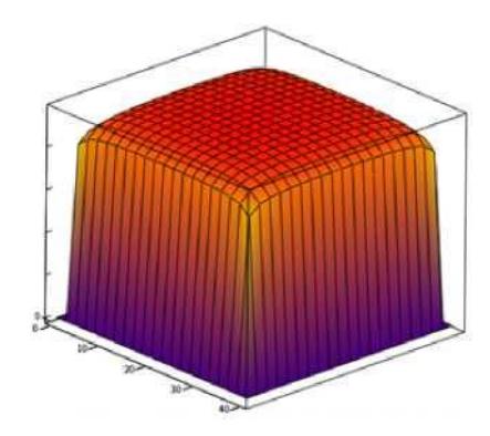
Figure 2 The distributed load as a double Fourier series, N = 40, M = 40.
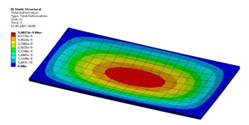
Figure 3 Deflection on the nanoplate. Result of the finite element analysis in ANSYS.
The Fourier series Eqs. (32a)-(32e), Eq. (33) were limited to the values of N and M for n and m, respectively. The distributed load q as a double Fourier series Eq. (33) for N = 40, M = 40 is shown in Figure 2. As we can see from Figure 2, the double Fourier series can represent a uniform load well enough.
The maximum plate deflection occurred in the plate's center and was equal to 5.0397∙10-9 m. According to numerical calculation in ANSYS with a 20-node hexahedron element that supported the third-order theory, the maximum plate's deflection was 5.0823∙10-9m (Figure 3). Thus, the difference between the solution in ANSYS and the present work was less than 0.8%.
The result of modeling in dimensionless variables is shown in Figure 4. In Figure 5, dimensionless deflections of the middle plane of the plate (x2 = L2/2) are shown.
3.2 Free Vibration
Natural frequencies of a simply supported orthotropic square microplate for different l3 are shown in Table 4 and the first five natural frequencies obtained in ANSYS are shown in Table 3.
Table 3 The first five natural frequencies (MHz) of a simply supported orthotropic square microplate obtained in ANSYS.
| Mode | Frequency, MHz |
|---|---|
| 1 | 1.785 |
| 2 | 2.336 |
| 3 | 3.305 |
| 4 | 4.556 |
| 5 | 4.669 |
| 6 | 5.077 |
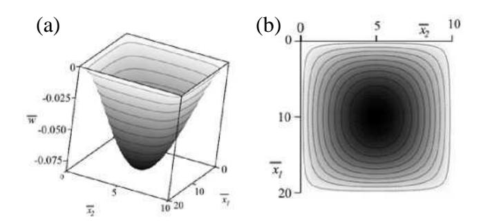
Figure 4 Dimensionless deflection of the plate, \(l_1 = \frac{1}{4h}\), \(l_2 = 0\): (a) isometric view (b) top view.
These results correspond to the results of other authors, in which the natural frequency of the plate also increased with an increase in the value of \(l_i\). It should be noted that the values of \(l_1\) and \(l_2\) do not affect the first natural frequency.
Table 5 lists the first two natural frequencies \(a_{nm}\) of a simply supported isotropic square microplate with various values of side-to-thickness ratio \(L_1/h = L_2/h = L/h\). The microplate was made of epoxy with the following material properties: E = 1.44 GPa, \(\rho = 1220\) Kg/m³, \(h = 3.52 \cdot 10^{-5} m\) [41]. The calculated frequencies were compared with those calculated using the expressions reported by Thai et al. [41] for size-dependent functionally graded thick plates based on the Mindlin plate theory and the modified couple stress theory. For comparison, these expressions were adapted for thin plates without nonlinearity.
Table 4 Natural frequencies of a simply supported orthotropic square microplate for different \(l_3\).
| n=1, | n=2, | n=1, | n=3, | n=1, | ||
|---|---|---|---|---|---|---|
| m = 1 | m = 1 | m = 2 | m = 1 | m = 3 | ||
| \(l_3 = 0\) | \(U_{nm}^0\) | 24.5899 | 46.9845 | 45.8241 | 60.4056 | 67.8134 |
| \(V_{nm}^{0}\) | 36.4089 | 30.8675 | 66.2657 | 39.5176 | 97.4348 | |
| \(W_{nm}^{0}\) | 1.8347 | 2.9847 | 6.0927 | 4.8641 | 12.9882 | |
| \(\Psi 1_{nm}^0\) | 429.3768 | 429.8315 | 434.1927 | 383.8177 | 442.0127 | |
| \(\Psi 2_{nm}^0\) | 380.1515 | 381.5337 | 382.0927 | 430.5897 | 385.324 | |
| \(l_3 = 0.5 \ h^{-1}\) | \(U_{nm}^0\) | 26.9187 | 46.991 | 55.6388 | 96.1344 | 60.4119 |
| \(V_{nm}^{0}\) | 36.416 | 34.2557 | 66.2907 | 97.8944 | 46.3156 | |
| \(W_{nm}^{0}\) | 1.8347 | 2.9848 | 6.0929 | 12.9888 | 4.8644 | |
| \(\Psi 1_{nm}^0\) | 408.2234 | 398.1097 | 430.1253 | 440.7786 | 395.8134 | |
| - | \(\Psi 2_{nm}^0\) | 448.2819 | 465.1479 | 494.6417 | 599.3565 | 498.6406 |
The solution presented here is in good agreement with the Navier solution presented in Ref. [41] for Mindlin plates and the modified couple stress theory.
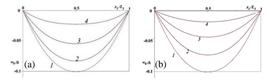
Figure 5 Dimensionless deflection of the plate, x2 = L2/2: (a) = , = ; (b) = = . − = ; − = ⁄; − = ⁄; − = ⁄.
Comparing these results with those obtained above, we can say that the modified couple stress theory and the modified strain gradient theory can predict different trends for different order plate theories for nonzero values of size-dependent parameters. Therefore, further study of the limits of applicability of both theories is necessary.
Table 5 Natural frequencies ( = 1, = 1), , of a simply supported isotropic square microplate for different 1/ℎ = 2/ℎ = /ℎ, = 0 .
| 𝑳/𝒉 | 40 | 60 | 80 | 100 | 200 | |
|---|---|---|---|---|---|---|
| First mode | [41] | 0.3284 | 0.2189 | 0.1642 | 0.1314 | 0.0657 |
| Current | 0.3284 | 0.2189 | 0.1642 | 0.1314 | 0.0657 | |
| Second mode | [41] | 0.5899 | 0.3932 | 0.2949 | 0.2359 | 0.1180 |
| Current | 0.5899 | 0.3932 | 0.2949 | 0.2359 | 0.1180 |
4 Conclusion
In this study, the bending and free vibration behavior of a rectangular nanoplate was investigated by considering the new modified couple stress theory and thirdorder shear deformation plate theory. The nanoplate was considered as a sizedependent thin orthotropic plate. The equations of motion of the nanoplate were obtained using Hamilton's principle. The natural boundary conditions were formulated
An analytical solution of the equations of motion of a simply supported nanoplate was constructed. The eigenvalue problem for the simply supported nanoplate was formulated and solved. The unknown components of displacement and rotation vectors were represented as double trigonometric rows. The constructed solution was verified by comparing the calculated results with the results of numerical plate modeling, carried out in one of the well-known complexes of finite element modeling, and with results obtained by other authors for low-order models of plates and bars. The obtained results can be used to simulate the stress-strain state of the sensitive elements of nano sensors, which are nanoplates.
It was shown that the displacements of the median surface points in the direction of the \(x_1\) and \(x_2\) axis do not depend on the material length scale parameter in the same directions. These displacements depend on the material length scale parameter in the \(x_3\) direction only. However, the deflection \(w_0\) does not depend on \(l_3\). Angles \(\phi_1\) and \(\phi_2\) depend on all length scale parameters. It was analytically shown that the size-dependent parameters have a noticeable effect on the deformed state of the plate only if their order is not less than order 1/h. Since the modified couple stress theory and the modified strain gradient theory can predict different trends for different order plate theories for non-zero values of size-dependent parameters, further study of the limits of applicability of both theories is necessary.
Acknowledgement
This research was funded by RFBR grant 19-08-00807.
Appendix A
\[\begin{split} &M_{1,1}=M_{2,2}=\rho h; \quad M_{3,3}=\frac{\rho h((\alpha^2+\beta^2)h+252)}{252}; \quad M_{4,4}=M_{5,5}=\frac{17\rho h^3}{315}; \\ &M_{3,4}=M_{4,3}=-\frac{4\rho\alpha h^3}{315}; \quad M_{3,5}=M_{5,3}=-\frac{4\rho\beta h^3}{315}; \\ &S_{1,1}^{cl}=h(C_{4,4}\beta^2+C_{1,1}\alpha^2); \quad S_{2,2}^{cl}=h(C_{2,2}\beta^2+C_{4,4}\alpha^2); \\ &S_{1,2}^{cl}=S_{2,1}^{cl}=h\beta\alpha(C_{1,2}+C_{4,4}); \\ &S_{3,3}^{cl}=\frac{h^3\cdot\left(C_{2,2}\cdot\beta^4+C_{1,1}\cdot\alpha^4+2\cdot\beta^2\cdot\alpha^2\cdot\left(C_{1,2}+2\cdot C_{4,4}\right)\right)}{15} \\ &+\frac{8\cdot h\cdot\left(C_{5,5}\cdot\beta^2+C_{6,6}\cdot\alpha^2\right)}{15} \\ &S_{3,4}^{cl}=\frac{8\cdot C_{6,6}\cdot\alpha\cdot h}{15}-\frac{4\cdot\beta\cdot h^3\cdot\left(\left(C_{12}+2\cdot C_{4,4}\right)\cdot\beta^2+C_{1,1}\cdot\alpha^2\right)}{315} \\ &S_{3,5}^{cl}=\frac{8\cdot C_{5,5}\cdot\beta\cdot h}{15}-\frac{4\cdot\beta\cdot h^3\cdot\left(C_{2,2}\cdot\beta^2+\left(C_{1,2}+2\cdot C_{4,4}\right)\cdot\alpha^2\right)}{315} \\ &S_{4,4}^{cl}=\frac{17\cdot h^3\cdot\left(C_{4,4}\cdot\beta^2+C_{1,1}\cdot\alpha^2\right)}{315}+\frac{8\cdot C_{6,6}\cdot h}{15} \\ &S_{4,5}^{cl}=\frac{17\cdot\beta\cdot\alpha\cdot h^3\cdot\left(C_{1,2}+C_{4,4}\right)}{315}; \quad S_{5,5}^{cl}=\frac{17\cdot h^3\cdot\left(C_{2,2}\cdot\beta^2+C_{4,4}\cdot\alpha^2\right)}{315}+\frac{8\cdot C_{5,5}\cdot h}{15} \\ &S_{1,1}^{ncl}=\frac{\beta^2\cdot h\cdot(\beta^2+\alpha^2)\cdot\xi_3}{4}; \quad S_{1,2}^{ncl}=-\frac{\beta\cdot\alpha\cdot h\cdot(\beta^2+\alpha^2)\cdot\xi_3}{4} \end{split}\]
\[\begin{split} S^{ncl}_{2,2} &= \frac{\alpha^2 \cdot h \cdot (\beta^2 + \alpha^2) \cdot \xi_3}{4} \\ S^{ncl}_{3,3} &= \left( -\frac{\alpha^2 \cdot (-3 \cdot h^2 \cdot (\beta^2 - \alpha^2) + 20)}{15 \cdot h} \cdot \xi_2 - \frac{\beta^2 \cdot (7 \cdot h^2 \cdot (\beta^2 - \alpha^2) + 20)}{15 \cdot h} \cdot \xi_1 \right. \\ &\quad + -\frac{14 \cdot \beta^2 \cdot \alpha^2 \cdot h \cdot (\xi_1 + \xi_2)}{15} \right) \\ S^{ncl}_{3,4} &= -\frac{2 \cdot \alpha \cdot (3 \cdot \alpha^2 \cdot h^2 - 10) \cdot \xi_2}{15 \cdot h}; \quad S^{ncl}_{3,5} &= -\frac{2 \cdot \beta \cdot (3 \cdot \beta^2 \cdot h^2 - 10) \cdot \xi_1}{15 \cdot h} \\ S^{ncl}_{4,3} &= \left( -\frac{2 \cdot \alpha^3 \cdot h}{3} - \frac{4 \cdot \alpha \cdot (2 \cdot \beta^2 \cdot h^2 - 5)}{15 \cdot h} \right) \cdot \xi_2 + \frac{\beta^2 \cdot \alpha \cdot h \cdot \xi_1}{15} \\ S^{ncl}_{5,3} &= \left( -\frac{\beta \alpha^3 \cdot h}{5} - \frac{4 \cdot \beta \cdot (2 \cdot \alpha^2 \cdot h^2 - 5)}{15 \cdot h} \right) \cdot \xi_1 + \frac{4 \cdot \beta \cdot \alpha^2 \cdot h \cdot \xi_2}{15} \\ S^{ncl}_{4,4} &= \frac{2 \cdot h^2 \cdot (\beta^2 + \alpha^2) + 20}{15 \cdot h} \cdot \xi_2 + \frac{\beta^2 \cdot h \cdot (17 \cdot h^2 \cdot (\beta^2 + \alpha^2) + 168)}{1260} \cdot \xi_3 \\ S^{ncl}_{5,5} &= \frac{2 \cdot h^2 \cdot (\beta^2 + \alpha^2) + 20}{15 \cdot h} \cdot \xi_1 + \frac{\alpha^2 \cdot h \cdot (17 \cdot h^2 \cdot (\beta^2 + \alpha^2) + 168)}{1260} \cdot \xi_3 \\ S^{ncl}_{5,4} &= -\frac{\beta \cdot \alpha \cdot h \cdot (17 \cdot h^2 \cdot (\beta^2 + \alpha^2) + 168) \cdot \xi_3}{1260} \\ S^{ncl}_{4,5} &= -\frac{\beta \cdot \alpha \cdot h \cdot (17 \cdot h^2 \cdot (\beta^2 + \alpha^2) + 168) \cdot \xi_3}{1260} \end{split}\]
Nomenclature
h = plate thickness
\(\rho_0\) = density
u = vector of displacements
\((u_0, v_0, w_0)\) = displacement components of a midplane point along the \((x_1, x_2, x_3)\)
coordinate axes
\(\phi_1\) = angle of rotation about the \(x_2\)-axis \(\phi_2\) = angle of rotation about the \(x_1\)-axis \(l_i\) = material length scale parameter
\(\tilde{C}_{ijkl}, G_i\) = elasticity constants \(\sigma, \varepsilon\) = stress and strain tensors
\(\chi\) = curvature (rotation gradient) tensor
m = couple stress moment tensor
e = permutation symbol (the Levi-Civita symbol)
CT = classical theory of plate deformation FOPT = first order theory of plate deformation TOPT = third order theory of plate deformation