
1 Introduction
African animal trypanosomiasis (AAT) is a parasitic disease caused by parasites of the genus Trypanosoma. The parasite lives in the blood, lymph, and various tissues in vertebrates. The main parasitic species that spread the disease are Trypanosoma congolense, Trypanosoma vivax and Trypanosoma brucei. AAT is transmitted by the blood-sucking tsetse fly, Glossina spp. The tsetse fly has a strong mouthpart that can penetrate thick skin (including rhino skin), namely the labium. The labium is the structure of the mouth of the tsetse fly, which consists of a series of tiny, sharp teeth that are capable of scraping thick skin. Thus, these flies can suck the host's blood easily [1]. Parasites carried over by fly bites live and multiply in the host's red blood cells [2].
AAT is one of the largest obstacles in controlling animal populations in tropical countries, especially in Africa. This is because parasite attacks by Trypanosoma are among the most common disease causes in the rhino population in South Africa, which includes white rhinos. The white rhino (Ceratotherium simum) is one of five rhino species that are not yet threatened with extinction. The World Wide Fund for Nature says that at the end of the nineteenth century, the southern white rhino subspecies was thought to have become extinct due to rampant poaching [3]. However, a small group of less than a hundred individuals was found in 1895 in Kwazulu-Natal, South Africa. This discovery initiated conservation practices to conserve the white rhino [3]. However, in 2012, the International Union for Conservation of Nature designated the white rhino as an endangered species with a declining population trend [4]. The difficulty of the white rhino population translocation program was exacerbated by the discovery of the AAT disease in the rhino population, especially those carried by Trypanosoma conglense, simiae, and godfreyi [5].
At first, AAT was considered to have a minor influence on white rhino population dynamics [6]. However, in the 1960s, researchers became aware of the fact that an AAT infection can become a real health threat for white rhinos when the animal is stressed [7]. Stress in rhinos can occur due to various factors, including overpopulation, lack of water and food, and anxiety [8]. AAT should be suspected if an animal in an endemic area is listless and in a problematic condition.
Based on the above and given that the white rhino is classified as Near Threatened [3], it is important to understand the impact of AAT on the population dynamics of white rhinos. Many authors have used different mathematical models to understand the population dynamics of a species affected by disease. Ref. [9] introduced an ecoepidemic mathematical model to understand the effect of disease on predators. They also considered prey group defense in their model. A mathematical model of disease in prey animals is discussed in [10]. Various types of incidence rates in an eco-epidemiological model are discussed in [11], where the possibility of Hopf bifurcation emerged from the proposed model. See [12- 15] for more references on ecoepidemiological models. Although many studies discuss ecoepidemiological models of predator-prey interaction or population dynamics models, few articles discuss mathematical models for AAT in rhino populations. For example, an earlier study on AAT and its intervention using insecticides and multi-host factors is presented in [16]. A mathematical model regarding human African trypanosomiasis was developed in [17], where the model was validated with real data. Recently, [18] introduced a fractional-order
model and optimal control problem for a human African trypanosomiasis model. They developed their model using a Susceptible-Infected-Recovered model on the human population and a Susceptible-Infected model on the vector population. Their numerical results showed that the combination of public education, effective treatment, and vector control as control measures succeeded in suppressing the spread of AAT in the human population. Ref. [19] analyzed a model of the spread of AAT in livestock by considering the use of insecticide. They constructed the basic reproduction number of their model with respect to the growth rate of infected wildlife around the susceptible population. They concluded that if treatment of cattle with insecticide did not take place, the wildlife would continue to be the source of infections in the livestock population. A model of the spread of AAT in livestock by considering treatment was introduced in [20]. Three immunity stages were included in the model, which revealed that it is possible that AAT may still exist even though the related reproduction number is smaller than one.
According to the references mentioned above, in this article, we consider a mathematical model for African animal trypanosomiasis. The novelty of this study lies in the involvement of infection detection and ground spraying on the rhino population. A mathematical model of the interaction between tsetse flies and rhinos has never been developed before. A detailed mathematical analysis was done to find the existence and local stability of equilibrium points. Using the Castillo-Song bifurcation theorem [21], we showed that our model may exhibit backward bifurcation at basic reproduction number equals one. To analyze the optimal intervention, we reconstructed our model as an optimal control problem. Pontryagin's maximum principle [22] was used to characterize the optimal condition of our problem. A cost-effectiveness analysis was conducted to determine the most cost-effective scenario for AAT intervention. Our numerical experiments on the optimal control problem indicated that a combination of ground spraying and infection detection will be successful in suppressing the spread of AAT in the rhino population. If a single intervention should be selected, then ground spraying is more cost-effective compared to infection detection.
This paper is structured as follows. The mathematical model that was constructed is discussed in detail in Section 2. The existence of all equilibrium points and their stability criteria are analyzed in Section 3, continued with a bifurcation analysis in Section 4. The sensitivity analysis and autonomous simulation to determine the elasticity of each parameter in our proposed model to the dynamics of the rhino and tsetse fly populations are discussed in Section 5 and also the basic reproduction number. The construction of the mathematical model for the optimal control problem is done in Section 6. Characterization, numerical simulations, and the cost-effectiveness of the optimal control problem are also discussed in Section 6. Finally, some conclusions are given in Section 7.
2 Mathematical model formulation
African animal trypanosomiasis (AAT) can be transmitted to rhinos through bites from tsetse flies. Here, we construct a novel mathematical model to describe the dynamics of AAT transmission among white rhino and tsetse fly populations. The model is based on a compartmental model with a system of non-linear ordinary differential equations. Therefore, our white rhino population is divided into five compartments based on their health status and their symptoms, namely, susceptible rhinos S(t), exposed rhinos E(t), undetected infected rhinos \(I_u(t)\), detected infected rhinos \(I_d(t)\), and recovered rhinos R(t). On the other hand, we divide the fly population into two compartments, namely, susceptible flies U(t)and infected flies V(t). We assume that due to the short life expectancy of flies, once a fly gets infected by parasites, the disease will be lifelong. Hence, we have the total population of rhinos denoted by \(N_r\), given by \(N_r(t) = S(t) + E(t) +\)\(I_u(t) + I_d(t) + R(t)\). On the other hand, the total population of flies, denoted by \(N_f\), is given by \(N_f(t) = U(t) + V(t)\). We construct our model based on the transmission diagram given in Figure 1, and the description of all parameters is given in Table 1.
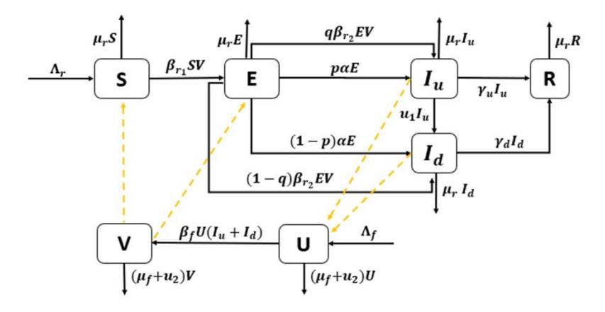
Figure 1 Transmission diagram of AAT in System (1).
Par. Description Unit Λℎ Recruitment rate of white rhinos ℎ Λ Recruitment rate of tsetse flies 1 Infection rate in white rhinos due to primary bites 1 × 2 Infection rate in white rhinos due to secondary bites 1 × Infection rate of tsetse flies 1 × ℎ Progression towards infected rhino compartment due to incubation period 1 Proportion of exposed rhinos who experience a secondary bite but do not show any symptoms (undetected) − Proportion of exposed rhinos who progress to infected rhinos after the incubation period but do not show symptoms (detected) − 1 Rate of infection detection 1 2 Rate of ground spraying 1 Recovery rate of infected undetected rhinos 1 Recovery rate of infected detected rhinos 1 Natural death rate of rhinos 1 Natural death rate of tsetse flies 1
Table 1 Description of parameters in model (1).
The construction of the model is as follows. We assume that all newborn (rate of Λ) are susceptible. We assume that AAT is not vertically transmitted through newborns. The number of susceptible rhinos then decreases due to primary bites from infected flies at a constant rate 1, and due to natural death at rate . In our model, we use a mass contact function to describe the infection process of AAT in the rhino and fly populations.
The number of exposed individual rhinos increases due to new infections from a susceptible compartment at a rate of 1 . This population can then decrease due to three reasons. The first is the constant natural death rate. The second is because of the disease's progression. After an incubation period of −1 , exposed rhinos will move to the infected compartment. However, since AAT does not always show symptoms, we have to add the $p$ portion of these individuals to the undetected cases and the rest (1 − ) to the detected cases. The last reason why the number of exposed rhinos decreases are secondary bites from flies, at a constant rate 2. Similarly, some proportion of the exposed rhinos () who do not show any symptoms will move to the undetected class, while 1 − goes to the detected class.
Due to detection efforts from the government to detect the existence of infection in white rhinos (at rate 1), there is a transition from the undetected infected to the detected infected rhino compartment. Furthermore, there is recovery of undetected and detected infected white rhinos at constant rates and , respectively. Note that due to additional treatment, we assume that ≥ . We presume that AAT does not cause any additional deaths in the infected white rhino population.
We assume that there is no vertical transmission in the population of tsetse flies. Hence, all recruitments go to susceptible flies (). Susceptible flies may get infected by AAT due to biting of infected white rhinos ( and ) at a constant rate of . In order to control the vector population, we include ground spraying at a constant rate of 2.
Based on the above description, the mathematical model of AAT transmission considering infection detection and ground spraying as interventions is given by the following system of ordinary differential equations.
\[\frac{dS}{dt} = \Lambda_r - \beta_{r1}SV - \mu_r S \tag{1a}\]
\[\frac{dE}{dt} = \beta_r SV - \alpha E - \beta_{r2} EV - \mu_r E, \tag{1b}\]
\[\frac{dI_u}{dt} = p\alpha E + q\beta_{r2} EV - u_1 I_u - \gamma_u I_u - \mu_r I_{u}, \tag{1c}\]
\[\frac{dI_d}{dt} = (1 - p)\alpha E + (1 - q)\beta_{r2}EV + u_1I_u - \gamma_dI_d - \mu_rI_d,\] (1d)
\[\frac{dR}{dt} = \gamma_u I_u + \gamma_d I_d - \mu_r R,\tag{1e}\]
\[\frac{dU}{dt} = \Lambda_f - \beta_f U(I_u + I_d) - (\mu_f + u_2)U, \tag{1f}\]
\[\frac{dV}{dt} = \beta_f U(I_u + I_d) - (\mu_f + u_2)V. \tag{1g}\]
Note that all parameters in System (1) are non-negative. In addition, System (1) is completed by the following non-negative initial condition:
\[S(0) > 0, E(0) \ge 0, I_u \ge 0, I_d \ge 0, R(0) \ge 0, U(0) > 0, V(0)\]
> 0. (2)
The following theorem guarantees that System (1) always has a unique solution and each solution is always non-negative as long as the initial condition is also non-negative.
Theorem 1. For any initial condition as in (2), System (1) has a unique solution for all time \(t \ge 0\).
Proof. The following inequality always holds:
\[\frac{dS}{dt} > -(\beta_{r1}V + \mu_r)S.\]
With the method of factor of integration, choosing \(\exp(\int_0^t (\beta_{r1}V(\tau) + \mu_r)d\tau)\) as the integration factor, and implementation into above equation, we have:
\[S(t) > S(0)\exp(-\int_0^t (\beta_{r1}V(\tau)d\tau + \mu_r t) > 0\] for all t > 0. From the above expression, we can see that \(\frac{dS}{dt}\) has a unique positive solution for a non-negative initial condition S(0). The existence and non-negativity of all other variables in System (1) can be shown in the same way. Hence, we can conclude that all solutions \(S, E, I_u, I_d, R, U\) and V are always non-negative for all time t > 0. Hence, the proof is completed.
In addition, we define the following feasible region of System (1):
\[\Gamma = \Gamma_r \times \Gamma_f,\] where
\[\Gamma_r = \left\{ (S, E, I_u, I_d, R) \in \mathbb{R}^5_+ : N_r \le \frac{\Lambda_r}{\mu_r} \right\}\] for the rhino population and
\[\Gamma_f = \left\{ (U, V) \in \mathbb{R}^2_+ : N_f \le \frac{\Lambda_f}{\mu_f + \mu_2} \right\}\] for the fly population. Using the same approach as in [23,24], we can show that \(\Gamma\) is positively invariant.
3 Existence and Stability of Equilibrium Points
3.1 The AAT-free Equilibrium and the Basic Reproduction Number
The ATT-free equilibrium point of System (1) is given by
\[\mathcal{E}_{1} = (S^{\dagger}, E^{\dagger}, I_{u}^{\dagger}, I_{d}^{\dagger}, R^{\dagger}, U^{\dagger}, V^{\dagger}) = \left(\frac{\Lambda_{r}}{\mu_{r}}, 0, 0, 0, 0, \frac{\Lambda_{f}}{\mu_{f} + u_{2}}, 0\right). \tag{3}\]
From the expression of \(S^{\dagger}\), we can see that the total population of rhinos in an AAT-free equilibrium only depends on the ratio between the recruitment rate and the natural death rate. On the other hand, the total population of flies depends not only on the recruitment rate and the natural death rate but also on ground spraying. Increasing ground spraying will reduce the number of flies in the equilibrium.
Next, we calculate the basic reproduction number of our model. The basic reproduction number (denoted by \(\mathcal{R}_0\)) defines the expected number of new cases caused by one primary case in a completely susceptible population during its infection period [25]. In many epidemiological models, the basic reproduction number determines the existence or disappearance of the disease. In several epidemiological models [26-30], the disease has a chance to die out from the population if the basic reproduction number is less than one and always exists if the basic reproduction number is larger than one. Using the next-generation method [31], the basic reproduction number of System (1) will be calculated as follows. The transmission (T) matrix and transition (\(\Sigma\)) matrix of the infected sub-compartment of System (1), which are evaluated at \(\mathcal{E}_1\), are given by
\[T = \begin{bmatrix} 0 & 0 & 0 & \frac{\beta_{r1}\Lambda_r}{\mu_r} \\ 0 & 0 & 0 & 0 \\ 0 & 0 & 0 & 0 \\ 0 & \frac{\beta_f\Lambda_f}{\mu_f + u_2} & \frac{\beta_f\Lambda_f}{\mu_f + u_2} & 0 \end{bmatrix},\] and
\[\Sigma = \begin{bmatrix} -pa - (1-p)\alpha - \mu_r & 0 & 0 & 0 \\ p\alpha & -u_1 - \gamma_u - \mu_r & 0 & 0 \\ (I-p)\alpha & u_1 & -\gamma_d - \mu_r & 0 \\ 0 & 0 & 0 & -\mu_f - u_2 \end{bmatrix},\]
respectively. Since T has a zero row, the next-generation matrix of System (1) can be calculated using the following formula:
\[K = -E^t T \Sigma^{-1} E,\] where \(E = \begin{bmatrix} 1 & 0 \\ 0 & 0 \\ 0 & 0 \\ 0 & 1 \end{bmatrix}\), and \(E^t\) is the transpose f E. Hence, the next generation matrix
\[K = \begin{bmatrix} 0 & -\frac{\beta_r \Lambda_r}{\mu_r (\mu_f + u_2)} \\ -\frac{\beta_f \Lambda_f p \alpha}{(\alpha + \mu_r)(u_1 + \gamma_u + \mu_r)(\mu_f + u_2)} + \frac{\beta_f \Lambda_f (p \gamma_u + p \mu_r - u_1 - \gamma_u - \mu_r) \alpha}{(\alpha + \mu_r)(u_1 + \gamma_u + \mu_r)(\gamma_d + \mu_r)(\mu_f + u_2)} & 0 \end{bmatrix}\]
The controlled basic reproduction number of System (1) is taken from the spectral radius of K, i.e.,
\[\mathcal{R}_{0} = \sqrt{\frac{\beta_{r1}\Lambda_{r}\beta_{f}\Lambda_{f}\alpha(p\gamma_{d} + (1-p)\gamma_{u} + u_{1} + \mu_{r})}{\mu_{r}(\mu_{f} + u_{2})^{2}(\alpha + \mu_{r})(u_{1} + \gamma_{u} + \mu_{r})(\gamma_{d} + \mu_{r})}}.\] (4)
Following the results on Theorem 2 in [32], we have the following theorem:
Theorem 2. The AAT-free equilibrium of System (1) is always locally asymptotically stable if \(\mathcal{R}_0 < 1\) and unstable if \(\mathcal{R}_0 > 1\).
The basic reproduction number \(\mathcal{R}_0\) in the context of our problem indicates the possibility of whether AAT will spread in the population or not. The consequence of Theorem 2 from an epidemiological point of view is that AAT has a possibility to be controlled and disappeared from the population as long as the value of \(\mathcal{R}_0\) is less than one. In many epidemiological models involving species interaction, basic reproduction plays an essential role in determining the existence of the disease. Keeping the basic reproduction number below one is enough to guarantee that the disease dies out. However, in some conditions, a basic reproduction number below one does not ensure the disappearance of the disease. We will discuss this in the following section.
The expression of \(\mathcal{R}_0^2\) from (4) can be rewritten as follows:
\[\mathcal{R}_0^2 = \underbrace{\left\{ \frac{\beta_{r1}}{\alpha + \mu_r} \frac{\Lambda_r}{\mu_r} \right\}}_{\widehat{\mathcal{K}}_1} \times \underbrace{\left\{ \frac{\beta_f}{\mu_f + u_2} \frac{\Lambda_f}{\mu_f + u_2} \right\}}_{\widehat{\mathcal{K}}_2} \times \underbrace{\left\{ \alpha \left( \frac{p\gamma_d + (1-p)\gamma_u + u_1 + \mu_r}{(u_1 + \gamma_u + \mu_r)(\gamma_d + \mu_r)} \right) \right\}}_{\widehat{\mathcal{K}}_2},\] where \(\mathcal{K}_1\) represents the total of expected new infected rhinos per fly, \(\mathcal{K}_2\) represents the total of expected new infected flies per rhino, and \(\mathcal{K}_3\) represents the effect of infection detection \(u_1\) and treatment for detected infected white rhinos \(\gamma_d\). Hence, we can see that to reduce \(\mathcal{R}_0\), we have to pay attention to these three components, because each of them represents a path of infection as well as the impact of intervention. For example, we can reduce \(\mathcal{R}_0\) by reducing the number of expected infected rhinos in terms of reducing the number of flies by ground spraying. We can also increase the infection detection rate and recovery rate of detected infected white rhinos in order to reduce \(\mathcal{R}_0\). Further discussion on the impact of each parameter in determining the size of \(\mathcal{R}_0\) will be discussed in Section 5.
3.2 AAT-endemic Equilibrium
In this section, we analyze the criteria for the existence of a nontrivial equilibrium point in System (1), namely the AAT-endemic equilibrium point \(\mathcal{E}_2\). The AAT-endemic equilibrium point represents a condition where all infected individuals are in equilibrium, which is given by:
\[\mathcal{E}_2 = (S^*, E^*, I_{1}^*, I_{d}^*, R^*, U^*, V^*), \tag{5}\] where
\[S^* = \frac{\Lambda_r}{V^* \beta_{r1} + \mu_r}, E^* = \frac{\beta_{r1} \Lambda_r V^*}{(V^* \beta_{r1} + \mu_r)(V^* \beta_{r2} + \alpha + \mu_r)'}\] \[I_u^* = \frac{\beta_{r1} \Lambda_r V^* (V^* q \beta_{r2} + a p)}{m_0}, I_d^* = \frac{\beta_{r1} \Lambda_r V^* m_1}{(\gamma_d + \mu_r) m_0'},\] \[R^* = \frac{\beta_{r1} \Lambda_r V^* m_2}{(\gamma_d + \mu_r) \mu_r m_0}, U^* = \frac{(\mu_f + u_2)(\gamma_d + \mu_r) m_0}{\Lambda_r \beta_f \beta_{r1} V^* m_3 + m_4},\] (6)
and
\[\begin{split} m_0 &= (\gamma_u + u_1 + \mu_r)(V\beta_{r1} + \mu_r)(V\beta_{r2} + \alpha + \mu_r), \\ m_1 &= -\big((q-1)\gamma_u + (q-1)\mu_r - u_1\big)V\beta_{r2} - \alpha((p-1)\gamma_u + (p-1)\mu_r - u_1), \\ m_2 &= \big((-V(q-1)\beta_{r2} - \alpha(p-1)\mu_r + (u_1 + \gamma_u)(V\beta_{9r2}) + \alpha)\big)\gamma_d \\ &\quad + \mu_r\gamma_u(Vq\beta_{r2} + \alpha p) \\ m_3 &= \beta_{r2} \left(\gamma_d q - q\gamma_u + \gamma_u + \mu_r + u_1\right), \\ m_4 &= \beta_f \left(\alpha, p\gamma_d - \alpha, p\gamma_u + \alpha\gamma_u + \alpha\mu_r + \alpha u_1\right)\Lambda_r \beta_{r1} \end{split}\]
Note that \(V^*\) is taken from the positive roots of the following second-degree polynomial:
\[F(V) = d_2V^2 + d_1V + d_0 = 0\] where
\[\text{[rumus tidak dapat ditampilkan dengan baik — lihat PDF asli]}\]
\[\begin{split} d_1^* &= \left( \mu_f + u_2 \right)^2 \mu_r^3 + \left( \mu_f + u_2 \right)^2 (\gamma_d + \gamma_u + \alpha + u_1) \mu_r^2 \\ &\quad + \left( \left( (\gamma_u + \alpha + u_1) \gamma_d + \alpha (u_1 + \gamma_u) \right) \mu_f^2 \right. \\ &\quad + \left( \left( (2\gamma_u + 2\alpha + 2 u_1) \gamma_d + 2\alpha (u_1 + \gamma_u) \right) u_2 + \Lambda_r \alpha \beta_f \right) \mu_f \\ &\quad + \left( \left( \gamma_u + \alpha + u_1 \gamma_d + \alpha (u_1 + \gamma_u) \right) u_2^2 + \Lambda_r \alpha \beta_f u_2 \right. \\ &\quad - \beta_{r2} \Lambda_f \Lambda_r \beta_f \right) \mu_r + \gamma_d \alpha (u_1 + \gamma_u) \mu_f^2 \\ &\quad + \alpha \left( 2\gamma_d (u_1 + \gamma_u) u_2 + (p\gamma_d + (-p+1) \gamma_u + u_1) \beta_f \Lambda_r \right) \mu_f \\ &\quad + \gamma_d \alpha (u_1 + \gamma_u) u_2^2 + (p\gamma_d + (-p+1) \gamma_u + u_1) \beta_f \Lambda_r \alpha u_2 \\ &\quad - \Lambda_f (q\gamma_d + (-q+1) \gamma_u + u_1) \beta_{r2} \beta_f \Lambda_r. \end{split}\]
From the expressions of \(d_2\) and \(d_0\), we can easily see that \(d_2\) is always positive, while \(d_0\) is negative if \(\mathcal{R}_0 > 1\). Therefore, we know that the multiplication of the root of F(V) will be negative if \(\mathcal{R}_0 > 1\). Hence, F(V) can always have exactly one positive root if \(\mathcal{R}_0 > 1\). We state this result regarding the existence of the AAT-endemic equilibrium in the following theorem:
Theorem 3. System (1) always has a unique AAT-endemic equilibrium if \(\mathcal{R}_0 > 1\).
Since F(V) is a second-degree polynomial, and Theorem 3 only guarantees the existence of \(\mathcal{E}_2\) when \(\mathcal{R}_0 > 1\) (not the opposite), it is possible that we may have another equilibrium when \(\mathcal{R}_0 < 1\). Furthermore, it is also possible that we have two AAT-endemic equilibriums for System (1). To analyze this, we use gradient analysis of V with respect to \(\mathcal{R}_0\) at \(\mathcal{R}_0 = 1\) and V = 0. Note that the condition of \(\mathcal{R}_0 = 1\) is qualitatively equivalent with \(\mathcal{R}_0^2 = 1\). Hence, for simplification purposes, instead of calculating \(\frac{\partial V}{\partial \mathcal{R}_0}\) at \(\mathcal{R}_0 = 1\), we will calculate \(\frac{\partial V}{\partial \mathcal{R}_0^2}\). An illustration of this gradient analysis can be seen in Figure 2.
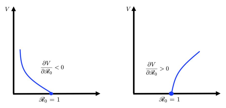
Figure 2 Illustration of \(\frac{\partial V}{\partial \mathcal{R}_0^2} < 0\) (left) and \(\frac{\partial V}{\partial \mathcal{R}_0^2} > 0\) (right). The left figure shows the existence of a positive root of F(V) when \(\mathcal{R}_0 < 1\). The right figure shows the existence of a positive root of F(V) when \(\mathcal{R}_0 > 1\)
To do this analysis, we should rewrite \(d_2\) and \(d_1\) in (7) as a function of \(\mathcal{R}_0^2\). Hence, since
\[\mathcal{R}_{0}^{2} = \frac{\beta_{r_{1}}\Lambda_{r}\beta_{f}\Lambda_{f}\alpha(p\gamma_{d} + (1-p)\gamma_{u} + u_{1} + \mu_{r})}{\mu_{r}(\mu_{f} + u_{2})^{2}(\alpha + \mu_{r})(u_{2} + \gamma_{u} + \mu_{r})(\gamma_{d} + \mu_{r})}.\] (8)
we can make \(\beta_{r1}\) a function of \(\mathcal{R}_0^2\) as follows:
\[\beta_{r1} = \mathcal{R}_0^2 \frac{\mu_r (\mu_f + u_2)^2 (\alpha + \mu_r) (u_1 + \gamma_u + \mu_r) (\gamma_d + \mu_r)}{\Lambda_r \beta_f \Lambda_f \alpha (p \gamma_d - p \gamma_u + u_1 + \gamma_u + \mu_r)}.\] (9)
Substituting \(\beta_{r_1}^*\) into F(V) in (7) and calculating the implicit differentiation of V with respect to \(\mathcal{R}_0^2\) yields:
\[\frac{\partial d_2}{\partial \mathcal{R}_0^2} V^2 + 2V d_2(\mathcal{R}_0^2) \frac{\partial V}{\partial \mathcal{R}_0^2} + \frac{\partial d_1}{\partial \mathcal{R}_0^2} V + \frac{\partial V}{\partial \mathcal{R}_0^2} d_1(\mathcal{R}_0^2) + \frac{\partial d_0}{\partial \mathcal{R}_0^2} = 0.\] (10)
Substituting \(\mathcal{R}_0 = 1\) and V = 0 to (10), and solving it with respect to \(\frac{\partial V}{\partial \mathcal{R}_0^2}\), we obtain:
\[\frac{\partial V}{\partial \mathcal{R}_0^2} = -\frac{\partial d_0}{\partial \mathcal{R}_0^2} \frac{1}{d_1 \mathcal{R}_0},\tag{11}\]
\[=2\mu_r(\mu_f+\mu_2)^2(\mu_1+\gamma_u+\mu_r)(\gamma_d+\mu_r)(\alpha+\mu_r)\frac{1}{d_1\mathcal{R}_0^2},\] (12)
where
\[d_1(\mathcal{R}_0^2 = 1) = c_0 - c_1 \,\beta_{r2},\tag{13}\] and
\[\begin{split} c_1 &= \, (\,\mu_r^2 + (\,(\,1-q\,)\gamma_u + q\gamma_d + u_1)\mu_r + \alpha(\,\gamma_d - \gamma_u)(\,q - p)\beta_f \Lambda_r \Lambda_f \\ c_0 &= (\,\mu_f + u_2)(\alpha + \mu_r)(\alpha p \Lambda_r \beta_f \gamma_d (\gamma_d - \gamma_u) + \alpha \Lambda_r \beta_f \gamma_u + \alpha \Lambda_r \beta_f \mu_r \\ &\quad + \alpha \Lambda_r \beta_f u_1 + \alpha \gamma_d \gamma_u \mu_f + \alpha \gamma_d \gamma_u u_2 + \alpha \gamma_d \mu_f \mu_r + \alpha \gamma_d \mu_f u_1 \\ &\quad + \alpha \gamma_d \mu_r u_2 + \alpha \gamma_d u_1 u_2 + \alpha \gamma_u \mu_f \mu_r + \alpha \gamma_u \mu_r u_2 + \alpha \mu_f \mu_r^2 \\ &\quad + \alpha \mu_f \mu_r u_1 + \alpha \mu_r^2 u_2 + \alpha \mu_r u_1 u_2 + \gamma_d \gamma_u \mu_f \mu_r + \gamma_d \gamma_u \mu_r u_2 \\ &\quad + \gamma_d \mu_f \mu_r^2 + \gamma_d \mu_f \mu_r u_1 + \gamma_d \mu_r^2 u_2 + \gamma_d \mu_r u_1 u_2 + \gamma_u \mu_f \mu_r^2 \\ &\quad + \gamma_u \mu_r^2 u_2 + \mu_f \mu_r^3 + \mu_f \mu_r^2 u_1 + \mu_r^3 u_2 + \mu_r^2 u_1 u_2. \end{split}\]
Let q > p, then we have \(\frac{\partial V}{\partial \mathcal{R}_0^2}|_{\mathcal{R}_0 = 1, V = 0} < 0\) if \(\beta_{r2} > \beta^{\ddagger}\), where \(\beta^{\ddagger} = \frac{c_0}{c_1}\). Based on the above analysis, we have the following theorem:
Theorem 4. System (1) has:
- 1. at least one positive AAT-endemic equilibrium for some \(\mathcal{R}_0 < 1\) if \(\beta_{r2} > \beta^{\ddagger}\)
- 2. no AAT-endemic equilibrium for all \(\mathcal{R}_0 > 1\) if \(\beta_{r2} < \beta^{\ddagger}\).
Based on Theorems 3-4 and using the concept of determinant of second-degree polynomials, we have the following corollary:
Corollary 1. Let \(\mathcal{R}_1 = \frac{d_1^2}{4d_2d_0}\) with \(d_0\), \(d_1\), and \(d_2\) is taken from the polynomial in Equation (7). Based on the condition of \(\mathcal{R}_1\), \(\mathcal{R}_0\), and \(\beta_{r2}\), System (1) has:
- 1. a unique AAT-endemic equilibrium if \(\mathcal{R}_0 > 1\)
- 2. no AAT-endemic equilibrium when \(\mathcal{R}_0 < 1\) and \(\beta_{r2} > \beta^{\ddagger}\)
- 3. no AAT-endemic equilibrium when \(\mathcal{R}_0 < \mathcal{R}_1 < 1\) and \(\beta_{r2} > \beta^{\ddagger}\)
- 4. two AAT-endemic equilibriums when \(\mathcal{R}_1 \leq \mathcal{R}_0 < 1\) and \(\beta_{r2} > \beta^{\ddagger}\).
See [33] for another approach of determining a condition for the existence of non-trivial equilibrium points for a second-degree polynomial equation. Based on the analysis in this section, it appears that the existence of a basic reproduction number that is smaller than one as an indicator of the disappearance of AAT can no longer always be guaranteed. This is because there is still a chance of the existence of AAT endemic equilibrium points even though the value of the basic reproduction number is smaller than one. In fact, it is possible to have two endemic equilibriums when the basic reproduction number is below one. This indicates the possibility of backward bifurcation in our model, which will be discussed in the following section. In our model, we can see that the possibility of backward bifurcation is triggered by secondary bites from flies to exposed rhinos (\(\beta_{r2}\)). Increasing the value of \(\beta_{r2}\) will increase the chance of the occurrence of backward bifurcation in our model. In the absence of secondary bites (\(\beta_{r2} = 0\)), we have \(d_1 = c_0 > 0\), which leads to the condition that \(\frac{\partial V}{\partial \mathcal{R}_0^2}\) is always positive. Hence, we have the following theorem:
Theorem 5. In the absence of secondary bites from flies to exposed rhinos (\(\beta_{r2} = 0\)), the AAT transmission model (1) has no AAT-endemic equilibrium when \(\mathcal{R}_0 \leq 1\) and always has a unique AAT-endemic equilibrium when \(\mathcal{R}_0 > 1\).
4 Backward bifurcation analysis
From the previous section, we see in Theorem 5 the possibility of the existence of two AAT-endemic equilibriums for some value of \(\mathcal{R}_0 < 1\). For many classical disease transmission models [34-36], the condition of a basic reproduction number less than one is enough to guarantee the disappearance of the disease. However, this condition is not always sufficient in the case of backward bifurcation, since the endemic equilibrium may co-exist with a disease-free equilibrium for some interval when the basic reproduction number is less than one. See [37-40] for some epidemiological models where backward bifurcation appears. Based on the above description, we conclude that backward bifurcation has significant implications for the success of interventions to control the spread of AAT.
In order to analyze the existence of backward bifurcation in our proposed AAT model in (1), we will use the well-known Castillo-Song theorem [21], which is based on the Center Manifold theory [41].
To apply the Castillo-Song Theorem to our model in (1), we make the following simplification. Let vector \(X = (x_1, x_2, x_3, x_4, x_5, x_6, x_7)\) and \(S = x_1, E = x_2, I_u = x_3, I_d = x_4, R = x_5, U = x_6, V = x_7\). Substituting these into System (1) yields:
\[g1 := \frac{dx_1}{dt} = \Lambda_r - \beta_{r1}x_1x_7 - \mu_r x_1,\] \[g2 := \frac{dx_2}{dt} = \beta_{r1}x_1x_7 - \alpha x_2 - \beta_{r2}x_2x_7 - \mu_r x_2,\] \[g3 := \frac{dx_3}{dt} = p\alpha x_2 + q\beta_{r2}x_2x_7 - u_1x_3 - \gamma_u x_3 - \mu_r x_3,\] \[g4 := \frac{dx_4}{dt} = (1 - p)\alpha x_2 + (1 - q)\beta_{r2}x_2x_7 - u_1x_3 - \gamma_d x_4 - \mu_r x_4,\] \[g5 := \frac{dx_5}{dt} = \gamma_u x_3 + \gamma_d x_4 - \mu_r x_5,\] \[g6 := \frac{dx_6}{dt} = \Lambda_f - \beta_f x_6(x_3 + x_4) - (\mu_f + u_2)x_6,\] \[g7 := \frac{dx_7}{dt} = \beta_f x_6(x_3 + x_4) - (\mu_f + u_2)x_7.\]
Now, let us choose \(\beta_{r1}\) as the bifurcation parameter. Hence, by solving \(\mathcal{R}_0^2 = 1\) with respect to \(\beta_{r1}\) gives us (the same argument as in the previous section is used in this section for \(\mathcal{R}_0^2 = 1\) instead of \(\mathcal{R}_0 = 1\)):
\[\beta_{r1}^{*} = \frac{\mu_r (\mu_f + u_2)^2 (\alpha + \mu_r) (u_1 + \gamma_u + \mu_r) (\gamma_d + \mu_r)}{\Lambda_r \beta_f \Lambda_f \alpha (p \gamma_d - p \gamma_u + u_1 + \gamma_u + \mu_r)}\](15)
Evaluating the eigenvalues of the Jacobian matrix of System (14) at AAT-free equilibrium gives us a simple zero eigenvalue, while the other six are negative. Due to its complex form, we do not explicitly show these six eigenvalues. Next, we need to determine the right and left eigenvectors of the Jacobian matrix that correspond to zero eigenvalue. We denote = [1 2 3 4 5 6 7] as the left eigenvector and = [1 2 3 4 5 6 7] as the right eigenvector. Then, we get:
\[v_{1} = 0,\] \[v_{2} = \alpha,\] \[v_{3} = \frac{(u_{1} + \mu_{r} + \gamma_{d})(\alpha + \mu_{r})}{p\gamma_{d} - p\gamma_{u} + u_{1} + \gamma_{u} + \mu_{r}},\] \[v_{4} = \frac{(u_{1} + \mu_{r} + \gamma_{u})(\alpha + \mu_{r})}{p\gamma_{d} - p\gamma_{u} + u_{1} + \gamma_{u} + \mu_{r}},\] \[v_{5} = 0,\] \[v_{6} = 0,\] \[v_{7} = \frac{(\gamma_{d} + \mu_{r})(\mu_{f} + u_{2})(\alpha + \mu_{r})(u_{1} + \mu_{r} + \gamma_{u})}{\Lambda_{f}\beta_{f}(p\gamma_{d} - p\gamma_{u} + u_{1} + \gamma_{u} + \mu_{r})},\] (16)
and
\[w_{1} = \frac{(\mu_{f} + u_{2})^{2}(\gamma_{d} + \mu_{r})(\alpha + \mu_{r})(u_{1} + \mu_{r} + \gamma_{u})}{(-p\gamma_{d} - \mu_{r} + (p - 1)\gamma_{u} - u_{1})\mu_{r}\alpha},\] \[w_{2} = \frac{(\mu_{f} + u_{2})^{2}(\gamma_{d} + \mu_{r})(u_{1} + \mu_{r} + \gamma_{u})}{(p\gamma_{d} - p\gamma_{u} + u_{1} + \gamma_{u} + \mu_{r})\alpha},\] \[w_{3} = \frac{p(\mu_{f} + u_{2})^{2}(\gamma_{d} + \mu_{r})}{(\gamma_{d} - \gamma_{u})p + u_{1} + \gamma_{u} + \mu_{r}},\] \[w_{4} = -\frac{((p - 1)\gamma_{u} + p\mu_{r} - u_{1} - \mu_{r})\mu_{r}\alpha(\mu_{f} + u_{2})^{2}}{(1 - p)\gamma_{u} + p\gamma_{d} + u_{1} + \mu_{r}},\] \[w_{5} = -\frac{(\mu_{f} + u_{2})^{2}(((p - 1)\mu_{r} - u_{1} - \gamma_{u})\gamma_{d} - p\mu_{r}\gamma_{u})}{((1 - p)\gamma_{u} + p\gamma_{d} + u_{1} + \mu_{r})\mu_{r}},\] \[w_{6} = -\Lambda_{f}\beta_{f},\] \[(17)\]
\[w_7 = \Lambda_f \beta_f\].
To determine the type of bifurcation of our Model (1) at ℛ0 = 1, we have to calculate and ℬ with the following formula:
\[\mathcal{A} = \sum_{k,i,j=1}^{7} v_k w_i w_j \frac{\partial^2 g_k}{\partial x_i \partial x_j} (0,0),\] \[\mathcal{B} = \sum_{k,i,j=1}^{7} v_k w_i \frac{\partial^2 g_k}{\partial x_i \partial \beta_{r1}} (0,0).\] (18)
To calculate and ℬ, we calculate the associated non-zero partial derivatives of , evaluated at ℰ1. The calculation is as follows:
\[\frac{\partial^2 g_2}{\partial x_7 \partial x_2} = \frac{\partial^2 g_2}{\partial x_2 \partial x_7} = -1, \frac{\partial^2 g_3}{\partial x_7 \partial x_2} = \frac{\partial^2 g_3}{\partial x_7 \partial x_2} = q \beta_{r2},\] \[\frac{\partial^2 g_4}{\partial x_7 \partial x_2} = \frac{\partial^2 g_7}{\partial x_2 \partial x_7} = (1 - q) \beta_{r2}, \frac{\partial^2 g_2}{\partial x_7 \partial x_1} = \frac{\partial^2 g_2}{\partial x_1 \partial x_2} = \beta_{r1},\] \[\frac{\partial^2 g_7}{\partial x_6 \partial x_3} = \frac{\partial^2 g_7}{\partial x_6 \partial x_4} = \frac{\partial^2 g_7}{\partial x_3 \partial x_6} = \frac{\partial^2 g_7}{\partial x_4 \partial x_6} = \beta_f.\]
Calculation of and . Using Eq. (18), we have:
\[\mathcal{A} = -\frac{2\beta_f (\mu_f + u_2)^2 (\gamma_d + \mu_r) (u_1 + \mu_r + \gamma_u) a^*}{(p\gamma_d - p\gamma_u + u_1 + \gamma_u + \mu_r)^2 \mu_r a},\] (19)
where ∗ is a positive expression, which is too long to be shown in this article.
On the other hand, the result for the calculation of ℬ is given by:
\[\mathcal{B} = \frac{\alpha \beta_f \Lambda_f \Lambda_r}{\mu_r} > 0. \tag{20}\]
From the above calculation, we can see that ℬ is always positive. On the other hand, can be positive or negative. After some algebraic calculations, we find that will be positive if 2 > ‡ , where ‡ is given the same critical parameter used in Theorem 4 and 5. With this result, we have the following theorem:
Theorem 6. The AAT model in (1) exhibits bifurcation at \(\mathcal{R}_0 = 1\) when \(\beta_{r2} > \beta^{\ddagger}\), and exhibits forward bifurcation if \(\beta_{r2} > \beta^{\ddagger}\).
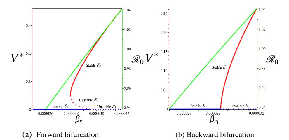
Figure 3 Two types of possible bifurcation of AAT in Model (1). The red figure is the plot of \(V^*\) in \(\mathcal{E}_2\) from polynomial (7), the blue figure is \(V^{\ddagger}\) in \(\mathcal{E}_1\), and the green figure is the plot of \(\mathcal{R}_0\) as a function of \(\beta_{r1}\). The dot and solid curve present unstable and stable equilibrium, respectively.
Figure 3 shows a numerical interpretation of Theorem 6. To conduct this numerical experiment we used the following parameter values:
\[\Lambda_r = \frac{1000}{50 \times 365}, \Lambda_f = \frac{1000}{30}, \mu_r = \frac{1}{50 \times 365}, \mu_f = \frac{1}{30}, p = 0.2\] \[\beta_{r1} = \frac{0.028}{1000}, \beta_f = \frac{0.028}{1000}, q = 0.5, \alpha = \frac{1}{51}, \gamma_u = \frac{1}{126}, \gamma_d = \frac{1}{63},\] \[u_1 = 0.01, u_2 = 0.01\] (21)
while \(\beta_{r2}\) varies depending on the condition of \(\beta^{\ddagger}\). Using the above parameters, we have \(\beta^{\ddagger}=0.085\). Hence, using Theorem 6, we choose \(\beta_{r2}=0.08<\beta^{\ddagger}\) to produce forward bifurcation at \(\mathcal{R}_0=1\) (Figure 3a), and \(\beta_{r2}=0.8<\beta^{\ddagger}\) to produce backward bifurcation at \(\mathcal{R}_0=1\) (Figure 3b). Note that we have multiple endemic equilibriums when \(\mathcal{R}_0<1\) in Figure 3b for \(\beta_{r1} \in [0.000027949, 0.000029529]\), which is equivalent to \(\mathcal{R}_0 \in [0.97287, 1]\). It can be seen that when forward bifurcation appears, then AAT always disappears whenever \(\mathcal{R}_0<1\), and starts to exist when \(\mathcal{R}_0<1\). On the other hand, we can see that when backward bifurcation appears, there still exists the possibility of a stable AAT-endemic equilibrium for some values of \(\mathcal{R}_0 < 1\). Hence, when backward bifurcation arises, controlling AAT not only relies on reducing \(\mathcal{R}_0\) to be smaller than one, but we should also consider the value of reinfection parameter \(\beta_{r2}\).
5 Sensitivity Analysis and Autonomous Simulation
In this section, we analyze the sensitivity of \(\mathcal{R}_0\) and our model to parameter change in System (1). Sensitivity analysis is essential to determine the qualitative behavior of \(\mathcal{R}_0\) toward each parameter and knowing which parameter is the most influential on our model. Several types of sensitivity analysis can be done regarding this, such as the Latin hypercube-partial rank correlation coefficient [42], the heat map method [43], and normalized forward sensitivity indices [44].
In this study, we used normalized forward sensitivity analysis to analyze the elasticity of \(\mathcal{R}_0\) with respect to each parameter in ATT model (1), using the following formula [44]:
\[\mathcal{E}_{\mathcal{R}_0}^P = \frac{\partial \mathcal{R}_0}{\partial P} \times \frac{P}{\mathcal{R}_0},\tag{22}\] where P is any parameter in AAT model (1). If \(\mathcal{E}_{\mathcal{R}_0}^P > 0\), then \(\mathcal{R}_0\) increases whenever P increases. On the other hand, we have \(\mathcal{R}_0\) decreases for an increase of P whenever \(\mathcal{E}_{\mathcal{R}_0}^P\). Using the expression of \(\mathcal{R}_0\) in (4) and the formula in (22), we have:
\[\mathcal{E}_{\mathcal{R}_0}^{\beta_{r_1}} = \frac{1}{2}\]
Then, increasing \(\beta_{r1}\) by 1% will increase \(\mathcal{R}_0\) for 0.5%. In addition, we also have:
\[\mathcal{E}_{\mathcal{R}_0}^{u_1} = \frac{(\gamma_d - \gamma_u)pu_1}{2(p\gamma_d(1-p)\gamma_u + u_1 + \mu_r)(\gamma_u + u_1 + \mu_r)'}\] which, when evaluated using the parameter values in (21), give us -0.023. On the other hand,
\[\mathcal{E}_{\mathcal{R}_0}^{u_2} = -\frac{u_2}{u_2 + \mu_f},\] which is equivalent to -0.231 when we use the parameter values in (21). Based on this result, we conclude that both interventions (infection detection and ground
spraying) have potential to reduce \(\mathcal{R}_0\). However, since \(|\mathcal{E}_{\mathcal{R}_0}^{u_1}| > |\mathcal{E}_{\mathcal{R}_0}^{u_2}|\), we can say that using the parameter values in (21), the ground spraying intervention is more effective in reducing AAT spread compared to infection detection. Using the same formula and parameter values, the elasticity of \(\mathcal{R}_0\) with respect to all parameters in System (1) is given in Table 2.
| \({\cal E}_{{\cal R}_0}^{\Lambda_r}\) | \(\mathcal{E}_{\mathcal{R}_0}^{\Lambda_f}\) | \(\mathcal{E}_{\mathcal{R}_0}^{\beta_{r_1}}\) | \(\mathcal{E}_{\mathcal{R}_0}^{\beta_{r_2}}\) | \(\mathcal{E}_{\mathcal{R}_0}^{\beta_f}\) | \(\mathcal{E}^\alpha_{\mathcal{R}_0}\) | \(\mathcal{E}_{\mathcal{R}_0}^{\mu_r}\) |
|---|---|---|---|---|---|---|
| 0.5 | 0.5 | 0.5 | 0 | 0.5 | 0.0014 | -0.503 |
| \(\mathcal{E}^P_{\mathcal{R}_0}\) | \({\mathcal E}^q_{{\mathcal R}_0}\) | \(\mathcal{E}_{\mathcal{R}_0}^{u_1}\) | \(\mathcal{E}_{\mathcal{R}_0}^{u_2}\) | \(\mathcal{E}_{\mathcal{R}_0}^{\gamma_u}\) | \(\mathcal{E}_{\mathcal{R}_0}^{\gamma_d}\) | \(\mathcal{E}_{\mathcal{R}_0}^{\mu_f}\) |
| 0.041 | 0 | -0.022 | -0.241 | -0.058 | -0.0417 | -0.769 |
Table 2 Elasticity of \(\mathcal{R}_0\) with respect to the parameters in System (1)
From Table 2, we can see clearly that \(u_1, u_2, \gamma_d, \gamma_u, \mu_r\), and \(\mu_f\) are inversely proportional to the change of \(\mathcal{R}_0\), while the other parameters are directly proportional to the change of \(\mathcal{R}_0\). Increasing \(u_1, u_2, \gamma_d, \gamma_u, \mu_r\), and \(\mu_f\) will reduce \(\mathcal{R}_0\). However, only the values of \(u_1, u_2\), and \(\gamma_d\) can be manipulated in the field to control the spread of AAT. Furthermore, we can see that the most influential parameter is \(\mu_f\), which indicates the potential of ground spraying or even genetic mutation to shorten the life expectancy of tsetse flies in order to reduce the spread of AAT through controlling the value of \(\mathcal{R}_0\). By substituting all parameter values in (21) (except \(u_1\) and \(u_2\)) into \(\mathcal{R}_0\), the contour plot of \(\mathcal{R}_0\) with respect to infection detection and ground spraying is given in Figure 4. We can see that increasing both interventions (infection detection and ground spraying) could reduce the magnitude of \(\mathcal{R}_0\). It was also confirmed that ground spraying is much more sensitive to \(\mathcal{R}_0\) than infection detection.
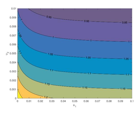
Figure 4 Level set of \(\mathcal{R}_0\) with respect to \(u_1\) and \(u_2\).
Based on the results of the elasticity analysis using the normalized forward elasticity analysis method, we next show the dynamic of solution of System (1) for the total infected rhino and infected fly populations for variations in the values of \(u_1\) and \(u_2\). The result can be seen in Figure 5. In Figure 5a, it can be seen that by increasing the value of infection detection interference \(u_1\), the dynamics of the infected rhino and fly populations decreased compared to when no infection detection intervention was given. However, it can be seen that a change in dynamic in both infected rhinos and flies for a value of \(u \in [0.0.1]\) did not provide a significant result. This is in line with the results of the elasticity calculation in Table 2, which shows that the elasticity of \(\mathcal{R}_0\) toward parameter \(u_1\) is relatively small, namely 0.022.
The autonomous simulation results regarding the total number of infected rhinos and flies in System (1) for various values of ground spraying intervention are given in Figure 5b. It can clearly be seen that ground spraying was much more effective in reducing the number of infected rhinos and flies than infection detection. This is in line with the elasticity analysis of the ground spraying intervention, which gave a relatively greater elasticity than the infection detection intervention, which was 0.231. In addition, it can also be seen that ground spraying at a sufficiently large intensity was able to prevent outbreaks of the number of infections in the rhino and fly populations.
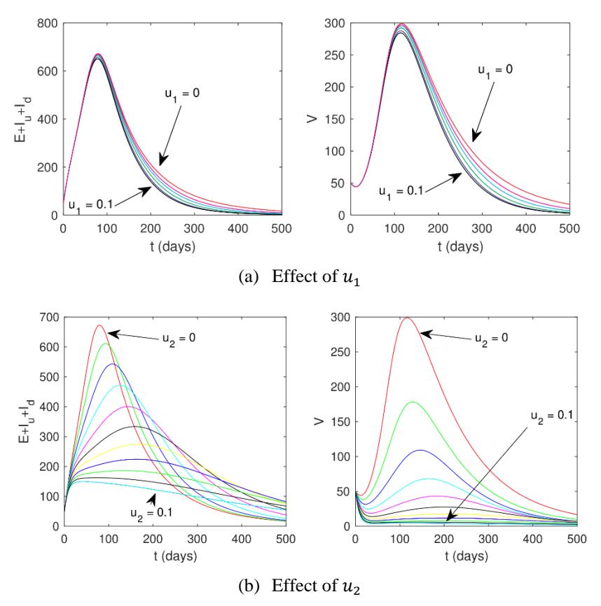
Figure 5 Effect of infection detection (a) and ground spraying (b) on the dynamic of total number of infected rhinos (left) and flies (right).
Based on Theorem 6, the AAT model in System (1) indicates that when ℛ0 < 1, there is a probability of AAT disappearing from the environment, and conversely the disease is always present in the environment when ℛ0 > 1. This result is illustrated by the autonomous simulation of System (1) for several different initial values of ℛ0 < 1 and ℛ0 > 1. The results can be seen in Figure 6. It shows that when ℛ0 < 1 and backward bifurcation does not occur, all initial values will go to the AAT-free equilibrium point. On the other hand, all solutions for all initial values will go to the AAT endemic equilibrium when ℛ0 > 1.
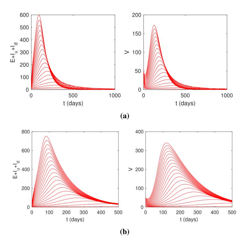
Figure 6 Simulations of System (1) for various initial conditions show a convergence of solutions of System (1) (total number of infected rhinos (left) and flies (right) to (a) an AAT-free equilibrium when \(\mathcal{R}_0 > 1\) and (b) an AAT-endemic equilibrium when \(\mathcal{R}_0 < 1\).
6 Optimal Control Problem
In the previous section, it was found that AAT disease in white rhino populations can be minimized (or even eliminated) if we can reach an \(\mathcal{R}_0 < 1\) condition. From the results of the sensitivity analysis of \(\mathcal{R}_0\), it can be seen that early detection and ground spraying have the potential to reduce the spread of AAT disease. The greater the intervention, the greater the reduction in the value of \(\mathcal{R}_0\) achieved. However, the high intensity of the intervention has the consequence of a high cost of implementation in the field. Therefore, it is deemed necessary that the interventions given are proportionate to the need. In this case, the infection detection and ground spraying should be treated as time-dependent variables. Based on this, the reconstruction of the model in System (1) to an optimal control model will be discussed in this section.
6.1 Characterization of the Optimal Control Problem
In order to construct our optimal control problem, we treat our constant intervention in System (1) as a time-dependent variable, i.e., \(u_1 = u_1(t)\), \(u_2 = u_2(t)\). Hence, System (1) now reads as follows:
\[\begin{split} \frac{ds}{dt} &= \Lambda_r - \beta_{r_1} SV - \mu_r S, \\ \frac{dE}{dt} &= \beta_{r_1} SV - p\alpha E - (1-p)\alpha E - q\beta_{r_2} EV - (1-q)\beta_{r_2} EV - \mu_r E, \\ \frac{dI_u}{dt} &= p\alpha E + q\beta_{r_2} EV - u_1(t)I_u - \gamma_u I_u - \mu_r I_u, \\ \frac{dI_d}{dt} &= (1-p)\alpha E + (1-q)\beta_{r_2} EV - u_1(t)I_u - \gamma_d I_d - \mu_r I_d, \\ \frac{dR}{dt} &= \gamma_u I_u + \gamma_d I_d - \mu_r R, \\ \frac{dU}{dt} &= \Lambda_f - \beta_f U(I_u + I_d) - \left(\mu_f + u_2(t)\right) U, \\ \frac{dV}{dt} &= \beta_f U(I_u + I_d) - \left(\mu_f + u_2(t)\right) V. \end{split}\]
Let us define the set of state variables as:
\[X = (S, E, I_u, I_d, R, U, V).\]
Our aim is to minimize the number of infected white rhinos and flies with intervention as low as possible. Hence, we define our objective function as follows:
\[\mathcal{J}(X, u_1, u_2) = \int_0^T (\omega_1 E + \omega_2 I_u + \omega_3 I_d + \omega_4 V + \varphi_1 u_1^2 + \varphi u_2^2) dt, \tag{24}\] where T is the final time of simulation, \(\omega_i\) for i=1,2,3,4 is the weight parameter for state variables E, \(I_u\), \(I_d\) and V, respectively, and \(\omega_j\) for j=1,2 is the weight parameter for the control variables \(u_1\) and \(u_2\), respectively. Note that
\[\int_0^T (\omega_1 E + \omega_2 I_u + \omega_3 I_d + \omega_4 V) dt\]
represents the total cost that is needed as a consequence of a high number of infected white rhinos and tsetse flies (except the cost for interventions). On the other hand,
\[\int_0^T (\varphi_1 u_1^2 + \varphi u_2^2) dt\]
represents the total cost of infection detection and ground spraying. For our model we choose a quadratic cost function in our objective function, which is common in epidemiological models [45-48].
Our optimal control problem is to seek a couple of controls \(u_1^*\) and \(u_2^*\) corresponding to state variable \(X^*\) on the interval [0,T]. In our case, the problem is to find the \(u_1^*\) and \(u_2^*\) that minimize the cost function (24) corresponding to state variable \(X^*\). Therefore, we want to find the minimum \(\mathcal{J}\), i.e.,
\[(X^*, u_1^*, u_2^*) = \lim_{\Gamma} \mathcal{J}(X, u_1, u_2),\] where
\(\Gamma = \{(u_1, u_2) | u_1 \text{ and } u_2 \text{ are Lebesgue integrable, with } 0 \le u_i \le 1 \text{, for } i = 1,2 \}\) as the admissible control set.
We derive the necessary condition for our optimal control problem using the well-known maximum principle of Pontryagin [22,49]. First, we define the Hamiltonian as follows:
\[\mathcal{H} = \omega_{1}E + \omega_{2}I_{u} + \omega_{3}I_{d} + \omega_{4}V + \varphi_{1}u_{1}^{2} + \varphi_{2}u_{2}^{*} + \lambda_{1}(\Lambda_{r} - \beta_{r_{1}}SV - \mu_{r}S) + \lambda_{2}(\beta_{r_{1}}SV - p\alpha E - (1 - p)\alpha E - q\beta_{r_{2}}EV - (1 - q)\beta_{r_{2}}EV - \mu_{r}E) + \lambda_{3}(p\alpha E + q\beta_{r_{2}}EV - u_{1}(t)I_{u} - \gamma_{u}I_{u} - \mu_{r}I_{d}) + \lambda_{4}((1 - p)\alpha E + (1 - q)\beta_{r_{2}}EV + u_{1}(t)I_{u} - \gamma_{d}I_{d} - \mu_{r}I_{d}) + \lambda_{5}(\gamma_{u}I_{u} + \gamma_{d}I_{d} - \mu_{r}R + \lambda_{6}(\Lambda_{f} - \beta_{f}U(I_{u} + I_{d}) - (\mu_{f} + u_{2}(t))U) + \lambda_{7}(\beta_{f}U(I_{u} + I_{d}) - (\mu_{f} + u_{2}(t))V),\] where \(\lambda_i\) for i = 1,2,...,7 are the adjoint variables. We have the following theorem as a consequence of Pontryagin's maximum principle:
Theorem 7. Given optimal control variables \(u_1^*\) and \(u_2^*\) that correspond to the optimal state variables \(X^* = (S^*, E^*, I_u^*, I_d^*, R^*, U^*, V^*)\), which minimize the cost function in (24), there exist adjoint variables that satisfy:
\[\frac{d\lambda_{1}}{dt} = \beta_{r_{1}}V(\lambda_{1} - \lambda_{2}) + \mu_{r}\lambda_{1},\] \[\frac{d\lambda_{2}}{dt} = -\omega_{1} + (p\alpha + q\beta_{r_{2}}V)(\lambda_{2} - \lambda_{3}) + ((1 - p)\alpha + (1 - q)\beta_{r_{2}}V)(\lambda_{2} - \lambda_{4}) + \mu_{r}\lambda_{2},\] \[\frac{d\lambda_{3}}{dt} = -\omega_{2} + u_{1}(\lambda_{3} - \lambda_{4}) + \gamma_{u}(\lambda_{3} - \lambda_{5}) + \beta_{f}U(\lambda_{6} - \lambda_{7}) + \mu_{r}\lambda_{3},\] \[\frac{d\lambda_{4}}{dt} = -\omega_{3} + \gamma_{d}(\lambda_{4} - \lambda_{5}) + \beta_{f}U(\lambda_{6} - \lambda_{7}) + \mu_{r}\lambda_{4},\] \[\frac{d\lambda_{5}}{dt} = \mu_{r}\lambda_{5},\] \[\frac{d\lambda_{6}}{dt} = \beta_{f}(I_{d} + I_{u})(\lambda_{6} - \lambda_{7}) + (\mu_{f} + u_{2})\lambda_{6},\] \[\frac{d\lambda_{7}}{dt} = -\omega_{4} + \beta_{r_{1}}S(\lambda_{1} - \lambda_{2}) + q\beta_{r_{2}}E(\lambda_{2} - \lambda_{3}) + (1 - q)\beta_{r_{2}}E(\lambda_{2} - \lambda_{4}) + (\mu_{f} + u_{2})\lambda_{7}.\] with a transversality condition \(\lambda_i(T) = 0\) for i = 1,2,...,7. Furthermore, the following functions characterize our optimal controls:
\[u_{1}^{*} = \max\left\{0, \min\left\{1, \frac{I_{d}(\lambda_{3} - \lambda_{4})}{2\varphi_{1}}\right\}\right\},\] \[u_{2}^{*} = \max\left\{0, \min\left\{1, \frac{\lambda_{6}U + \lambda_{7}V}{2\varphi_{2}}\right\}\right\}.\] (27)
Proof. The result of this theorem is a direct consequence of Pontryagin's maximum principle [22,49]. Taking the negative of the partial derivative of the Hamiltonian function (25) with respect to each state variable gives us:
\[\frac{d\lambda_1}{dt} = -\frac{\partial \mathcal{H}}{\partial S}, \frac{d\lambda_2}{dt} = -\frac{\partial \mathcal{H}}{\partial E}, \frac{d\lambda_3}{dt} = -\frac{\partial \mathcal{H}}{\partial I_u}, \frac{d\lambda_4}{dt} = -\frac{\partial \mathcal{H}}{\partial I_d}, \frac{d\lambda_5}{dt} = -\frac{\partial \mathcal{H}}{\partial R}, \frac{d\lambda_6}{dt} = -\frac{\partial \mathcal{H}}{\partial U}, \frac{d\lambda_7}{dt} = -\frac{\partial \mathcal{H}}{\partial V},\] (28)
with the transversality condition () = 0 for = 1,2, … ,7. Taking the partial derivative of ℋ with respect to each control variable yields:
\[\begin{split} \frac{\partial \mathcal{H}}{\partial u_1} &= 2\varphi_1 u_1 - I_d (\lambda_4 - \lambda_3), \\ \frac{\partial \mathcal{H}}{\partial u_2} &= 2\varphi_2 u_2 - \lambda_6 U - \lambda_7 V. \end{split}\]
Solving ℋ 1 = 0 and ℋ 2 = 0 with respect to 1 and 2, respectively, we have:
\[u_1^{\dagger} = \frac{I_d(\lambda_3 - \lambda_4)}{2\varphi_1}, \quad u_2^{\dagger} = \frac{\lambda_6 U + \lambda_7 V}{2\varphi_2}.\]
Due to the limited capability to implement the control variables, we chose that each control variables should be in the interval of [0, 1]. Therefor we have:
\[u_{1}^{*} = \max\left\{0, \min\left\{1, \frac{I_{d}(\lambda_{3} - \lambda_{4})}{2\varphi_{1}}\right\}\right\},\] \[u_{2}^{*} = \max\left\{0, \min\left\{1, \frac{\lambda_{6}U + \lambda_{7}V}{2\varphi_{2}}\right\}\right\}.\] (29)
This completes the proof.
To sum up, our optimal control problem consists of the state system (23) with a non-negative initial condition (2), adjoint system (26) with a transversality condition () = 0 for = 1,2, … ,7, cost function (24), and the optimal control conditions (27).
6.2 Numerical Experiments
In this subsection, we solve our optimal control problem using a forwardbackward iterative method [49]. Several authors have used this method in different types of epidemiological models [50-52]. First, using an initial guess for the control variables, we solve the state system (23) forward in time numerically.
With this result, we sole our adjoint system (26) backward in time with the transversality condition given. We update our control variables using the formula in (27). The iterative process continues until a convergence criterion is satisfied. To conduct our simulation, we use the same parameter values as in (21), while the weight parameters are \(\omega_1 = \omega_2 = \omega_3 = 1\), \(\omega_4 = 0.01\), \(\varphi_1 = \varphi_2 = 10^4\).
6.2.1 Endemic prevention vs endemic reduction scenarios
The first numerical experiment was conducted based on a different initial condition of System (23). Based on this assumption, we had two scenarios, namely an endemic prevention scenario and an endemic reduction scenario. In the endemic prevention scenario, the initial condition of infected white rhinos and tsetse flies was relatively small compared to the total populations. For our case, we chose the following initial condition for the endemic reduction scenario:
\[IC_1 = [S(0), E(0), I_u(0), I_d(0), R(0), U(0), V(0)] = [950, 20, 30, 0, 0, 960, 0].\]
The result of optimal control for the endemic prevention scenario is given in Figure 7. From the numerical experiments in Figure 7, it can be seen that the success of the time-dependent interventions of infection detection and ground spraying prevents the number of infected rhinos in compartment E and \(I_u\), and infected flies V from increasing. The number of infected rhinos in \(I_d\) increases not because of failure of the controls, but because of the infection detection intervention, which brings the rhinos in \(I_u\) to \(I_d\). We can see that the infection detection intervention is monotonically increasing at the beginning of the simulation period, massively reducing the number of undetected infected rhinos. After reaching its peak, it will decrease to zero until the end of the simulation. Unlike the infection detection intervention, the ground spraying intervention produced a higher rate at the beginning of the simulation period. It decreased rapidly in the early period and decreased slower when the number of infected flies was already small. The cost of intervention for this scenario was 10,721.3.
The next simulation was the endemic reduction scenario, which is characterized by a high number of infected rhinos and flies at t = 0. The following initial condition is given:
\[IC_2 = [S(0), E(0), I_{11}(0), I_{12}(0), R(0), U(0), V(0)] = [800, 20, 180, 0, 0, 800, 200].\]
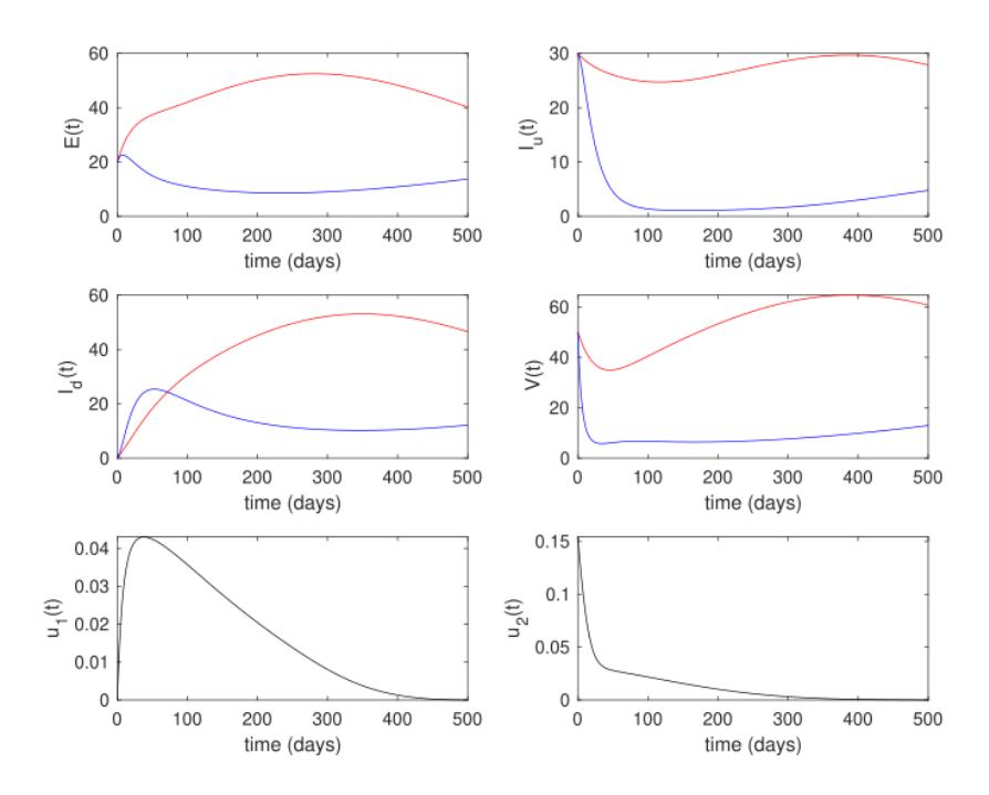
Figure 7 White rhinos, tsetse flies, and control trajectories under the endemic prevention scenario.
The optimal control results are given in Figure 8. Although the profile of controls in the endemic reduction scenario was somewhat similar in the endemic prevention scenario (high at the beginning and monotonically decreasing after the infected population decreased), it is clear that a higher intensity of intervention should be given in the endemic reduction scenario. This should be done to reduce the number of infected rhinos and flies as soon as possible. As a consequence, the cost of endemic reduction was much higher than in the endemic prevention scenario, i.e., 35,942.4 (more than three times larger).
Based on the numerical experiments in this section, it can be concluded that preventing the spread of AAT from the outset is easier, because it requires lower intervention costs. If the number of infections is already high at the start of a new intervention, then the intensity of the intervention must be relatively high from the start. This results in high intervention costs for endemic reduction cases.
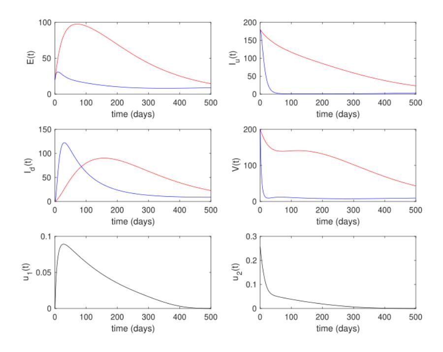
Figure 8 White rhinos, tsetse flies, and control trajectories under the endemic reduction scenario.
6.2.2 Different combinations of interventions
Unlike in the previous subsection, numerical scenarios will be carried out based on the type of combination of interventions used in this subsection. The scenarios are divided into three, namely when both interventions are given (first scenario), when infection detection is a single intervention (second scenario), and when ground spraying is a single intervention (third scenario). To conduct the simulation in this section, we used initial condition IC1 for all scenarios.
Figure 7 shows the numerical result for the first scenario. As already explained in the previous subsection, both interventions succeed in suppressing the number of infected rhinos and flies almost during the whole simulation, except for the number of detected infected rhinos. This glitch occurred due to the high intensity of early detection at the beginning of the simulation.
The result for the second strategy is given in Figure 9. It can be seen that when the policymakers only rely on infection detection to prevent the spread of AAT, the result is not as good as in the first scenario. It can be seen that the reduced
number of infected rhinos and flies was not as high as in the first scenario. However, the cost of intervention for the second scenario was much lower than for the first scenario, i.e., only 5,781.9, almost twice smaller than in the first scenario.
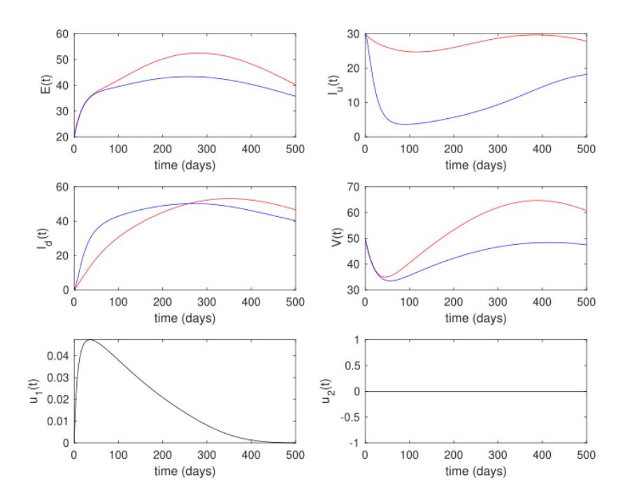
Figure 9 White rhinos, flies and control trajectories under the intervention strategy of the second scenario (1 () ≥ 0, 2 () = 0).
In the last simulation, which involved the third scenario, ground spraying was the only intervention implemented. The results are given in Figure 10. It can be seen that the control trajectories of 2 in the third scenario were somewhat similar with the first scenario, i.e., high intensity should be implemented at the beginning and decrease when the number of infected flies starts decreasing. As a result, the number of infected rhinos and flies decreased much more compared to the second scenario, but not as much as in the first scenario. The cost of intervention for the third scenario was 6,320.1.
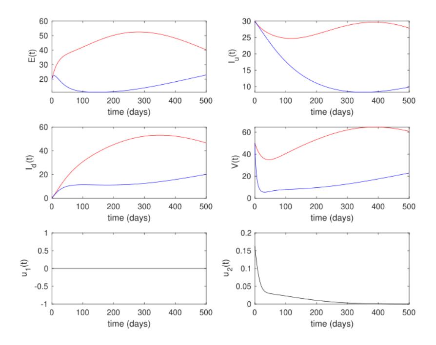
Figure 10 White rhinos, tsetse flies and control trajectories under the intervention strategy of the third scenario (1 () = 0, 2 () ≥ 0).
Cost-effectiveness analysis. From the numerical experiments with all of the above scenarios, it can be seen that all scenarios provided a reduced number of infected rhinos and flies. However, a good result comes with high intervention costs. Hence, we have to determine which is the best strategy compared to the other in terms of cost-effectiveness. To do this, we used two types of costeffectiveness measures, namely the Average Cost-Effectiveness Ratio (ACER) and the Incremental Cost-Effectiveness Ratio (ICER).
The ACER method aims to determine which strategy produces the lowest average cost for each reduction of one infected individual. The formula for calculating the ACER value is as follows:
\[ACER = \frac{Total\ cost\ for\ intervention}{Total\ number\ of\ infection\ averted} \tag{30}\]
A lower ACER value indicates a better result. A low ACER value means that the average cost for each infected rhino averted is also small. The result of the ACER analysis is given in Figure 11. From Figure 11, we can see that intervention of ground spraying as a single intervention was more cost-effective compared to the others, followed by the first and the second scenario, respectively.
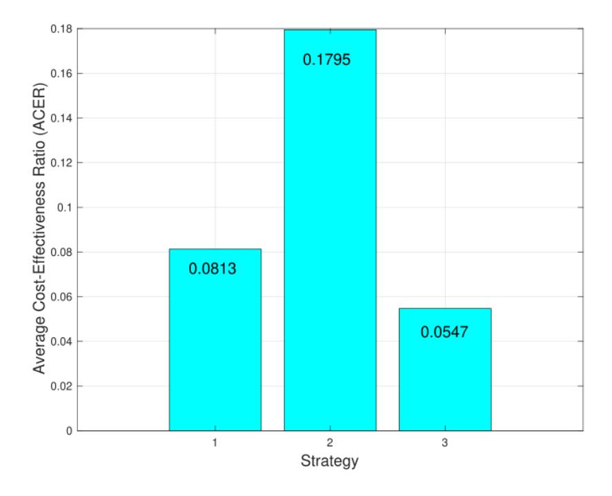
Figure 11 The result of ACER analysis.
The second method used to analyze the cost-effectiveness of the above strategies was the Incremental Cost-Effectiveness Ratio (ICER) method. This method aims to find the best strategy from two compared strategies. The following equation expresses the formula:
\[ICER_{i-j} = \frac{Difference\ of\ cost\ between\ strategy-i\ and\ j}{Difference\ of\ \#\ of\ infection\ averted\ between\ strategy-i\ and\ j} \tag{31}\]
First, we rank our strategies from the smallest number of infected rhinos averted to the highest number of infected rhinos averted for each strategy. The result is given in Table 3.
| Strategy | Total infections | Total cost | ICER | |
|---|---|---|---|---|
| nd scenario 2 | averted 32 210.2 | 5 781.9 | 0.1795 | |
| rd scenario 3 | 115 489.7 | 6 320.1 | 0.00646 | |
| st scenario 1 | 131 833.9 | 10 721.3 | 0.269 | |
Table 3 All scenario in increasing order based on the number of rhino infections averted.
Since ICER-2 > ICER-3, we eliminate the second scenario for the next calculation. Hence, we can conclude that the second scenario was the least costeffective strategy based on the ICER analysis. For the next calculation, we compare the third with the first scenario. The result is given in Table 4. Since ICER-1 > ICER-3, we can conclude that the third strategy, i.e., the implementation of ground spraying as a single intervention, is the best strategy. This result is in line with our previous analysis using the ACER method.
Table 4 Comparison between third and first scenarios
| Strategy | Total infection averted | Total cost | ICER |
|---|---|---|---|
| rd scenario 3 | 115 489.7 | 6 320.1 | 0.05 |
| st scenario 1 | 131 833.9 | 10 721.3 | 0.269 |
7 Conclusion
A large number of reports have noted the emergence of African Animal Trypanosomiasis (AAT) in the Nearly Threatened white rhino population. Thus, qualitative research related to efforts to minimize the spread of AAT is important, requiring serious attention from various parties, including mathematicians. Therefore, this article introduced a mathematical model for AAT, involving populations of white rhinos and tsetse flies, and two interventions, namely infection detection and ground spraying. Mathematical model analysis showed how the AAT-free equilibrium point is always locally asymptotically stable when the basic reproduction number is less than one. On the other hand, it is possible to have multiple AAT-endemic equilibriums when the basic reproduction number is less than one. A unique AAT-endemic equilibrium always exists when the basic reproduction number is larger than one. Bifurcation analysis using the Castillo-Song theorem [21], showed the possibility of backward bifurcation emerging from our model. Hence, there is a situation when the basic reproduction number being less than one is not enough to guarantee the disappearance of AAT from the population [37-40]. Sensitivity analysis of the basic reproduction number showed that infection detection and ground spraying both have potential to suppress the spread of AAT. However, we found that ground spraying is more
effective in influencing the basic reproduction number's size than infection detection.
From numerical simulations of the optimal control problem, it was found that time-dependent interventions successfully reduced the spread of AAT in the white rhino and tsetse fly populations. The cost-effectiveness analysis found that ground spraying as a single intervention is a better strategy than infection detection as a single intervention or a combination between infection detection and ground spraying. In addition, we also found that preventive interventions are more advisable to save on intervention costs rather than waiting for a high number of infections and then implementing interventions.
This research showed that AAT can significantly influence the dynamics of white rhino populations. To suppress the spread of AAT, ground spraying is highly recommended as a single intervention to prevent possible endemics.
Acknowledgement
This research was financially supported by RistekBRIN, Indonesia through the PDUPT Research Grant Scheme 2021 (ID number: NKB-165/UN2.RST/HKP.05.00/2021).