
1 Introduction
Inversion of geophysical data is essential for subsurface interpretation of processed field data responses. Inversion is physio-mathematical fitting of computed responses to measured data. Currently, inversion algorithms have been specifically developed for modeling electromagnetic data, for example, Occam inversion for EM sounding data by Constable et al. [1] and the Marquardt algorithm using using Singular Value Decomposition by Widodo & Saputera [2]. Since the One-dimensional (1D) inversion of EM data differs in the depth direction, it is essential in the interpretation of multidimensional models.
A TDEM field campaign is an active method that uses an artificial current source. There are two fundamental principles of TDEM measurement: Lenz's and Faraday's laws. The current injected in the transmitter produces a magnetic field.
A secondary magnetic field is generated by the eddy current when the current turns off suddenly in the conductive subsurface according to Maxwell's equations. The induced voltage of the secondary magnetic field is measured in the receiver.
According to Pellerin & Wannamaker [3], TDEM is effective in instigating a good conductor at depth, however, it is less sensitive in mapping resistivity anomalies in the low conductivity range. There are many applications of TDEM. It has been applied in hydrogeological studies [4,5], mineral exploration [6], and many more fields, ranging in scale from a few meters to several kilometers. In geological structure investigation, the TDEM technique gave good results in mapping the near surface fault structure in Mygdonian Basin [7].
The inversion model of TDEM data gives the subsurface geological parameters. To solve the inversion problem in TDEM data, many different inversion techniques can be applied, such as transient electromagnetic sounding, which uses a rapid inversion developed by Eaton and Hohmann [8], Direct inversion of TDEM data by Nekut [9], or the Laterally Constrained Inversion (LCI) algorithm by Christiansen et al. [10].
A hybrid variant of the FPA and elitism algorithms(eFPA) could be an alternative method to solve inversion problems of TDEM data. The simulation done by Yang [11] summarizes the FPA algorithm. The application of FPA in geophysical modeling has been conducted by Sungkono [12] to overview modeling of selfpotential (SP) data and 1D vertical electrical sounding (VES) data by Raflesia & Widodo [13].
In order to test the algorithms, FPA and eFPA were applied to approximate imaging of the subsurface response of TDEM data. The forward and inversion algorithms were executed using the Matlab Programming Language. The full source code is available in Appendix A (inverse modeling), Appendix B (forward modeling), and Appendix C (Levy distribution). Improvement and modification of the script is welcomed.
2 Methods
2.1 Forward Modeling
In TDEM measurement, the vertical component magnetic field is used and the time derivative of the secondary magnetic field can be denoted as follows[14]:
\[\frac{\partial H_z}{\partial t} = -\frac{I}{\mu_0 \sigma a^3} \left[ 3 \text{erf}(\theta a) - \frac{2}{\sqrt{\pi}} \theta a (3 + 2\theta^2 a^2) e^{-\theta^2 a^2} \right] \tag{1}\]
\[\theta = \sqrt{\frac{\mu_0 \sigma}{4t}} \tag{2}\]
\[\operatorname{erf}(x) = \frac{1}{\sqrt{\pi}} \int_{-x}^{x} e^{-t^2} dt\] (3)
where is the loop radius, is the current, and is the conductivity of the earth. Due to decay of transients, the distribution of time can be distinguished into early and late times.
The calculations in the inversion program need a proper forward modeling method. We used Adaptive Born Forward Mapping [15,16] for the TDEM forward modeling. The use of this forward modeling method has also been carried out for Central Loop Time Domain Electromagnetic Inversion using the Levenberg-Marquardt algorithm. This method uses the Born series, which defines a function that changes linearly as the model is updated from the reference model . The first order of the Born series is used as the function approximation.
\[G(m) = G(m^0) + \int \mathcal{F}'(m^0, r)[m(r) - m^0(r)]dr\] (4)
is the Fréchet kernel from the function, and is an unchanged variable from the Fréchet kernel. The reference model (0 ) can be expressed as:
\[G(m^0) = \int \mathcal{F}'(m^0, r)(m^0(r))dr\] (5)
Thus, Equation 4 becomes:
\[G(m) = \int \mathcal{F}'(m^0, r)(m(r))dr \qquad (6)\]
The Adaptive Born approximation is calculated based on the apparent conductivity of the constant half-space conductivity 0 → corresponds to the Fréchet kernel in Equation (4). Exchanging Equations (4) and (6) to equation (7) becomes
\[\sigma_{\mathbf{a}}(t) = \int_{0}^{\infty} \mathcal{F}'(\sigma_{\mathbf{a}}(t), z, t) (\sigma(z)) dz\] (7)
This equation is called Adaptive Born Forward Mapping instead of Ordinary Born Approximation. In the discrete problem, Equation 7 is formulated as:
\[\sigma_{a}(t_{i}) = \sum_{i=1}^{L} \sigma_{i} \mathcal{F}_{ij} \qquad (8)\]
The apparent conductivity () at time , is decay time, and is the conductivity model for the layer ( .
Christensen [15] has formulated an analytic Fréchet kernel to calculate apparent conductivity, although the formula is not sufficient to approximate the conductivity response from TDEM. Therefore, approximation of the Fréchet kernel is done:
\[\mathcal{F}\left(z_{j}, t_{i}, \sigma_{a}(t_{i})\right) = \begin{cases} \frac{z_{j}}{D_{i}} \left(2 - \frac{z_{j}}{D_{i}}\right), & \text{for } z_{j} \leq D_{i} \\ 1, & \text{for } z_{j} > D_{i} \end{cases}\] \[(9)\] with
\[D_i = \sqrt{\frac{c \cdot t_i}{\mu_0 \sigma_a(t_i)}}\] \[\tag{10}\] is a constant of the sensitivity of the Fréchet kernel. This whole process of apparent conductivity calculation is done by using iteration. The function in Equation (9) is an approximate forward mapping. The weighted sum of conductivities of each layer is denoted by:
\[\sigma_a^{k+1} = \alpha \, \sigma_a^{k+1} + (1 - \alpha) \, \sigma_a^k \tag{11}\]
To gain stability of the calculation, single exponential smoothing is applied. Using Equation 11, the apparent conductivity from the iteration is calculated using the apparent conductivity from the iteration with weighting constant .
Based on a trial-and-error process, the number of iterations that gives adequate results is 20. The transient can be estimated using Equation 1.
2.2 Inversion Method
FPA simulates the fertilization process of flowers. Fertilization can be done through self-fertilization or cross-fertilization (Figure 1). Self-fertilization is the union of female and male gametes of the same plant. It reduces the genetic diversity, while cross fertilization is the fusion of female and male gametes of different plants of the same species. Crossfertilization increases genetic diversity.
Figure 1 Flower fertilization: (1) and (2) self-fertilization, and (3) cross- fertilization from different plants [13].
The fertilization technique can be divided into global and local schemes. Global fertilization can be expressed as:
\[s_i^{t+1} = s_i^t + \alpha L(\lambda)(s_i^t - gbest)\] (12)
Local fertilization can be expressed as:
\[s_i^{t+1} = s_i^t + \in (s_j^t - s_k^t)\] (13)
where, , , is the fertilization of dissimilar individuals of the same species. Each index is different, , while ∈ signifies a uniform distribution between 0 and 1.
Greedy selection can be expressed as [13]:
\[s_i^{t+1} = \begin{cases} s_i^{t+1} & \text{if } f(s_i^{t+1}) \le f(s_i^t) \\ s_i^t & \text{if } f(s_i^{t+1}) > f(s_i^t) \end{cases}\] (14)
The elitism strategy produces the most suitable individuals among the candidates for selection [21]. It is a smooth method of increasing randomization, in which the best successor solutions are kept (and bad ones are replaced) to carry over to the next iteration. The overall eFPA is summarized in Figure 2. The total population used is 100.
1. Define a switch probability p \in [0,1];
2. Initialize the randomly generated population within its upper and lower
   bounds:
3. Calculate objective function of pollen using Eq. (16);
4. Find the best solution gbest in the initial population;
5. while abs(min_{RMS}-max_{RMS}) > 10^{-10} \&\& min_{RMS} > 10^{-10} \&\& iteration < 1000;
6.
          for i=1:n (n indicates number of pollen);
7.
                        rand <p;
8.
                         global pollination via Eq. (12);
9.
                  else
10.
                         do local pollination via Eq. (13);
11.
                  end if
12.
                  Evaluate new solutions;
13.
                  Use greedy selection Eq. (14);
14.
                Find the current worst solution and replace (elitism)
15.
          end for
16.
          Identify the present best solution gbest;
17. end while
Figure 2 Pseudo-code of eFPA.
The minimum function aims to obtain a response model that matches the observed data. It is denoted as the square root of the prediction error, which represents the misfit between the measured data, \(d_i\) and the model data, m, with standard deviation \(\sigma_i\). The data misfit is obtained by monitoring the root mean square (RMS) error as [17]:
\[E_{RMS} = \sqrt{\frac{1}{N} \sum_{i=1}^{N} \left[ \frac{d_i - f_i(m)}{\sigma_i} \right]^2 x 100}\] (15)
3 Results
In order to get an appropriate model, the testing algorithms used multi-layer models. The best and worst models were created after ten FPA and eFPA runs in each study, for which the products from the number of iterations and success rates are displayed in table 1. In the calculation of TDEM data approximation, a transmitter current of 1 Ampere was used, a loop radius of 25 m with sampling number at 20 and sampling time at 1 – 1 .
3.1 Synthetic Data
A synthetic model was calculated using the analytic equations from the previous sections. Three starting models were used in the forward model estimation. The first was a homogeneous layer with 100 , the second model was a more resistive layer with 100 m depth and 10000 resistivity. The third model was a more conductive layer with 100 m depth and 1 resistivity (Figure (b)
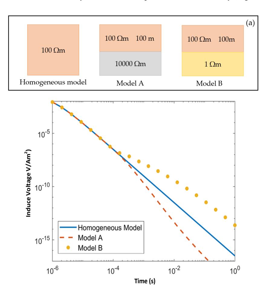
Figure 3 (a) Sketch of synthetic model, (b) TDEM response time derivative.
The transient responses of the multi-layer models are shown in Figure 3b. The homogeneous half space model gave a constant response. Initially, the transient of model A had the same feature as the transients of the homogeneous and B
models, while the curve decayed to a lower value at 10-4 s at the end, since the there was a resistive layer in the second layer. This lower value indicates that the decaying magnetic field was slower than the homogeneous one. The curve trend changes of the more resistive second layer shows a smoother curve compared to the less resistive layer in the second layer (Model B). The result reveals that the TEM method is capable of detecting the conductive target layer beneath the resistive overburden. Figure 4 shows the apparent resistivity results versus time.
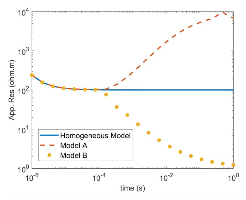
Figure 4 Curve of apparent resistivity versus time.
Table 1 Inverse results from synthetic data.
| Model | Parame | True | Space | FPA | eFPA | |||
|---|---|---|---|---|---|---|---|---|
| ter | Value | Min | Max | Best | Worst | Best | Worst | |
| Homog | ρ (𝛺m) | 100 | 1 | 20000 | 100 | - | 100 | - |
| eneous | Number of iterations | 561-908 | 178-478 | |||||
| Model | Number of iterations Success rate | 10/10 | 10/10 | |||||
| Model A | ρ1 (𝛺m) | 100 | 1 | 20000 | 100.18 | 101.05 | 99.97 | 100.84 |
| ρ2 (𝛺m) | 10000 | 10002.58 | 10117.14 | 9999.71 | 9961.25 | |||
| h1 (m) | 100 | 1 | 500 | 100.11 | 101.61 | 99.99 | 100.99 | |
| Number of iterations | 1000 | 425-701 | ||||||
| Success rate | 10/10 | 10/10 | ||||||
| Model B | ρ1 (𝛺m) | 100 | 1 | 20000 | 100 | - | 100 | - |
| ρ2 (𝛺m) | 1 | 1 | - | 1 | - | |||
| h1 (m) | 100 | 1 | 500 | 100 | - | 100 | - | |
| Number of iterations | 1000 | 457-760 | ||||||
| Success rate | 10/10 | 10/10 | ||||||
Furthermore, the results of the forward modeling were inverted using FPA and eFPA to see the ability of these two algorithms in synthetic data processing. Table 1 presents the true model parameters, true value, search space, best result, worst result, number of iterations, and success rate. FPA and eFPA resulted in 10 times the global minimum solution out of 10 runs. The modeling of the inversion results from the synthetic model only shows model A because it had different values. The results of the inversion of model A can be seen in Figure 5, consisting of the true value, best and worst result of FPA and eFPA.
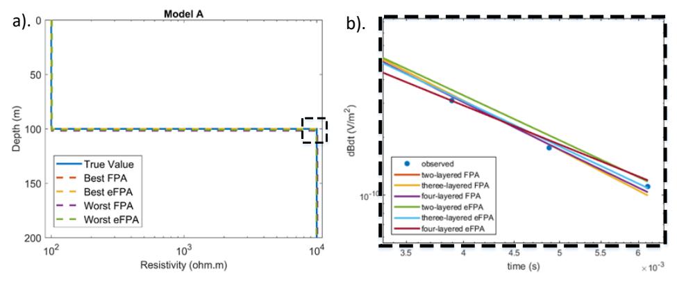
Figure 5 (a) Resistivity of model A; (b) the black dashed line indicates the magnification of Figure 5(a).
3.2 Field Data
The TDEM data were obtained in the epicenter area of the 1978 earthquake in the Volvi and Langada Lakes, Thessaloniki. This is a seismic active area, which has produced complex geological structures. The research was done by Widodo [7] using radiomagnetotelluric (RMT) and TDEM data to investigate the nearsurface structure. The field campaigns were carried red using a Zonge device. Later, these data were employed in the inversion process using two, three and four-layers.
Figure 6a shows the transient of the TDEM data and its inversion results from three different starting model layers (two, three and four layers of the starting model, respectively). This technique was applied to obtain the final model. The transients gave a similar response to one another. In order to get the best model in terms of the number of layers, magnification was carried out on Figure 6a in Figure 6b. The magnified view indicates that an initial model with four layers of gave better fitting. This means that the sum of the layers of the initial models will be influenced by the final model.
Figure 7 shows inversion models of the TDEM field data for the three different initial starting models. The model resistivity of each sounding was calculated
using two, three and four layers of the initial model. The results of FPA and eFPA in the two-layered model show the same resistivity and thickness values. Meanwhile, the three- and four-layered models show different values.
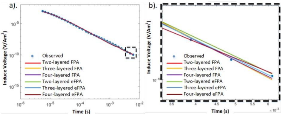
Figure 6 (a) Transient of TDEM field data using three different starting models; (b) the red square in the zoom view in Figure 6(b) shows the separated curves for each layer.
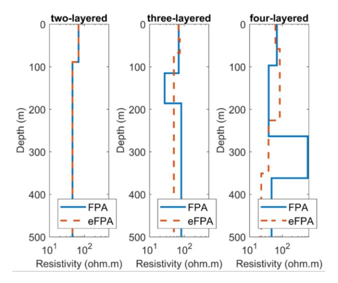
Figure 7 Resistivity model from field data
4 Discussion
Unlike the homogeneous model and model B, model A shows different values. Although it did not show the same results for the true value, the inverse results of the synthetic data from eFPA were better than FPA. In addition, the number of iterations required for eFPA was less than for FPA. FPA had more difficulty to achieve convergence, so in model A and model B the number of iterations was limited to 1000.
Figure 8a shows the comparison of the RMS errors between FPA and eFPA. FPA produced the lowest value (7.69%). The results of FPA and eFPA for the twolayered model had the same relative root mean square error values. Meanwhile, the three- and four-layered models had different values. The eFPA relative RMS error value was smaller than that of FPA for the three-layered model and the fourlayered model.
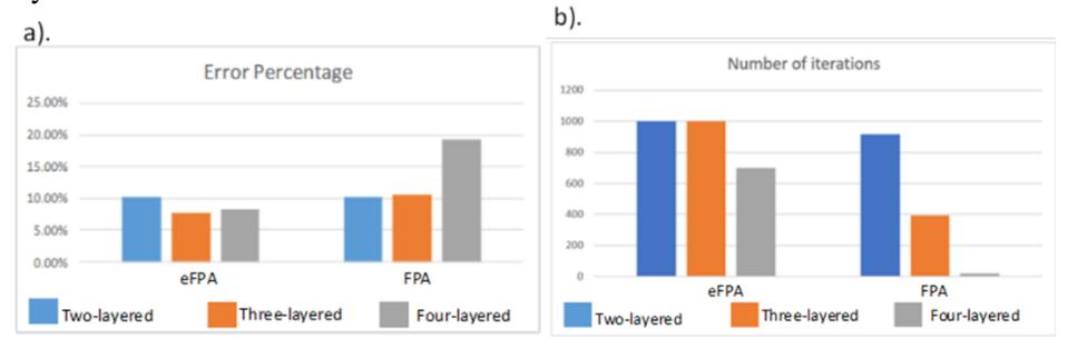
Figure 8 The performance of FPA and eFPA: (a) RMS errors of the three different starting models, (b) FPA and eFPA.
The total number of iterations for inversion modeling of the TDEM data using FPA and eFPA algorithms can be seen in Figure 8b. The algorithm of eFPA produced sufficiently competitive results against FPA'sstrategy, which improved the quality of the fitting data. Since eFPA enhances elitism capability, the inversion results produced better model results.
5 Conclusions
This research used a variant of the FPA and eFPA algorithms that focuses on improving the inversion of TDEM data. Algorithm testing is a time-consuming process, which can be minimized by using different search-based algorithms to meet certain coverage sizes. Hybridization of the algorithms (FPA and eFPA) gave good results in TDEM data inversion. FPA and eFPA could solve synthetic as well as field TDEM data. The provisions of the inversion process need more attention, especially for eFPA schemes.
6 Acknowledgement
We would like to thank to LPPM, PPMI Project, Institut Teknologi Bandung (ITB), and Riset Terapan Grant, RISTEK DIKTI.
7 References
[1] Constable, S.C., Parker, R.L. & Constable, C.G., Occam's inversion: A practical algorithm for generating smooth models for elecctromagnetic sounding data, Geophysics, 52, pp. 289-300, 1987.
- [2] Widodo, W. & Saputera, D. H., Improving Levenberg-Marquardt Algorithm Inversion Result Using Singular Value Decomposition, Earth Sci. Res. https://doi.org/10.5539/esr.v5n2p20. 2016.
- [3] Pellerin, L. & Wannamaker, P. E., Multi-dimensional electromagnetic modelling and inversion with application to near-surface earth investigations, Computers and Electronics in Agriculture, 46, 71-102. 2005.
- [4] Porsani, J.L., Bortolozo, C.A., Almeida, E.R., Sobrinho, E.N.S. & Santos, T.G. (2012) TDEM Survey in Urban Environmental for Hydrogeological Study at USP Campus in São Paulo City, Brazil. Journal of Applied Geophysics, 76, 102-108. https://doi.org/10.1016/j.jappgeo.2011.10.001, 2012.
- [5] Ibraheem, I. M., El-Qady, G. M. & ElGalladi, A., Hydrogeophysical and structural investigation using VES and TDEM data: A case study at El-Nubariya–Wadi El-Natrun area, west Nile Delta Egypt NRIAG, J. Astron. Geophysics. 5(1), 198-215. https://doi.org/10.1016/j.nrjag.2016.04.004, 2016.
- [6] Zhenwei, G., Guoqiang, X., Jianxin, L. & Xin, W., Electromagnetic methods for mineral exploration in China (Review), Ore Geology Reviews, 118. https://doi.org/10.1016/j.oregeorev.2020.103357, 2020.
- [7] Widodo, Tezkan, B. & Gurk, M., Multidimensional Interpretation of Radiomagnetotelluric and Transient Electromagnetic Data Measured in The Mygdonian Basin, Northern Greece, Journal Engineering and Geophysics, 21(3), 121-133, 2016.
- [8] Eaton, P.A. & Hohmann, G.W., A rapid inversion technique for transient electromagnetic soundings, Phys. Earth Plan. Int. 53, 384-404, 1989.
- [9] Nekut, A. G., Direct inversion of time-domain electromagnetic data, Geophysics, 52, pp. 1431-1435 (15), 1987.
- [10] Christiansen, A. V., Auken, E., N, Foged & Sorensen, K.I., Mutually and laterally constrained inversion of CVES and TEM data: A case study, Near Surface Geophysics, 115-123, 2007.
- [11] Yang, X.S., Flower pollination algorithm for global optimization, in: Lecture Notes in Computer Science (Including Subseries Lecture Notes in Artificial Intelligence and Lecture Notes in Bioinformatics), htttps://doi.org/10.1007/978-3-642-32894-7_27, 2012.
- [12] Sungkono, Robust interpretation of single and multiple self-potential anomalies via flower pollination algorithm, Arabian Journal of Geoscience, 13, 100, 2020.
- [13] Raflesia, F. & Widodo. W., Flower pollination algorithm for the inversion of Schlumberger sounding curve, in: The 3rd Southeast Asian Conference on Geophysics, IOP Conf. Ser.: Earth Environ. Sci. 873 012018, 2021.
- [14] Christensen, N. B., Imaging of Central-Loop Transient Electromagnetic Soundings, Journal of Environment and Engineering Geophysics, 1, 53-66, 1995.
- [15] Christensen, N. B., A Generic 1-D Imaging Method for Transient Electromagnetic Data, Geophysics, 67, 438-447, 2002.
- [16] Yogi, I.B.S., & Widodo, Central Loop Time domain electromagnetic inversion based on Born Approximation and Lavenberg-Marquardt Algorithm, IOP Conference Series: Earth and Environmental Science, 62, https://aip.scitation.org/doi/abs/10.1063/1.4990901, 2017.
- [17] Jackson D. D., Interpretation of inaccurate, insufficient, and inconsistent data, Geophysical Journal of Royal and Astronomical Society 28 97, 1972.
Appendix A
close all;
clear all;
clc;
tic
format long;%load data
load datahomo.dat;
dBdt=datahomo(1,:);
nl=2; %number of layers
nt=nl-1;
npop=100; %total population
prp=0.8; %probability
Lbr=[1 1]; %search space [lower bound resistivity]
Ubr=[20000 20000]; %search space [upper bound resistivity]
Lbt=[1]; %search space [lower bound thickness]
Ubt=[500];
rmseror=[];
t=linspace(log10(10^-6),log(1),20);
t=10.^t;
a=25;
I=1;
for i=1:npop
 popr(i,:)=Lbr+(Ubr-Lbr).*rand(1,nl);%popr=population of resistivity
 popt(i,:)=Lbt+(Ubt-Lbt).*rand(1,nt); %popt=population of thickness
 R=popr(i,:);
 thick=popt(i,:);
[dBdtc]=forwardloop(R,thick,t,a,I);
rms(i)=norm((dBdtc./dBdt)-1)/sqrt(length(dBdtc))*100; %root mean square
(percentage)
end
mr=min(rms); %rms minimum
mrm=max(rms); %rms maximum
q=find(rms==mr); %find rms minumum from population members
gRbest=popr(q,:); %best resistivity value
gthickbest=popt(q,:); %best thickness value
iteration=0;
while abs(mr-mrm) > 1E-20 && mr > 1E-9
 iteration=iteration+1;
 for i=1:npop
 if rand<prp
 n=1;
 m=nl;
 beta=1.5;
 [L]=levy(n,m,beta);%levy distribution
 npopr(i,:)=popr(i,:)+(0.1.*L.*(popr(i,:)-gRbest(1,:))); % Update the
new solutions
 npopr(i,:)=max(npopr(i,:),Lbr); %keep resistivity always in search
space
 npopr(i,:)=min(npopr(i,:),Ubr); %keep resistivity always in search
space
 m=nt;
 [L]=levy(n,m,beta);
 npopt(i,:)=popt(i,:)+(0.1.*L.*(popt(i,:)-gthickbest(1,:))); % Update
the new solutions
 npopt(i,:)=max(npopt(i,:),Lbt); %keep thickness always in search
space
 npopt(i,:)=min(npopt(i,:),Ubt); %keep thickness always in search
space
 else
 epsilon=rand;
 JK=randperm(npop);
 npopr(i,:)=popr(i,:)+epsilon*(popr(JK(1),:)-popr(JK(2),:));
 % Check the simple limits/bounds
 npopr(i,:)=max(npopr(i,:),Lbr);
 npopr(i,:)=min(npopr(i,:),Ubr);
 npopt(i,:)=popt(i,:)+epsilon*(popt(JK(1),:)-popt(JK(2),:));
 % Check the simple limits/bounds
 npopt(i,:)=max(npopt(i,:),Lbt);
 npopt(i,:)=min(npopt(i,:),Ubt);
 end
 R=npopr(i,:);
 thick=npopt(i,:);
[dBdtc]=forwardloop(R,thick,t,a,I);
nrms=norm((dBdtc./dBdt)-1)/sqrt(length(dBdtc))*100; %root mean square
(percentage)
 % If rms errors ok, update then
 if (nrms<=rms(i))
 popr(i,:)=npopr(i,:);
 popt(i,:)=npopt(i,:);
 rms(i)=nrms;
 end
 if nrms<mr
 gRbest=popr(i,:);
gthickbest=popt(i,:);
mr=nrms;
 end
 end
C=1./R;
for k=1:20
ac=mean(C)*ones(1,(length(t)));
 %elitism
 mrm=max(rms);
qq=find(rms==mrm);
popr(qq(end),:)=gRbest;
popt(qq(end),:)=gthickbest;
rmseror(iteration)=mr;
end
figure(1)
plot(t,dBdt,'*r')
hold on
plot(t,dBdtc)
set(gca,'Xscale','log');
set(gca,'Yscale','log');
ylim([10^-17 10^-2]);
xlabel('time (s)');
ylabel('dBdt');
legend('obs.','cal.','location','southwest');
figure(2)
rhoplot=[0,gRbest];
thkplot=[0,cumsum(gthickbest),max(gthickbest)*1000];
stairs(rhoplot,thkplot,'--','LineWidth', 2)
ylim([0 max(gthickbest)*2]);
xlim([0.1 2000]);
set(gca,'Ydir','reverse');
set(gca,'Xscale','log');
xlabel('Resistivity (ohm.m)');
ylabel('Depth (m)');
save('dataBnaik1eFPA.txt','dBdtc', 'rmseror','gRbest','gthickbest','iteration','mr','-
ascii')
Appendix B
%Function loop1d
function[dBdtc]=forwardloop(R,thick,t,a,I)
format long;
u0=4*pi*10^(-7);
c=1.2;
alpa=0.4;
depth=cumsum(thick);
 d=sqrt((c*t)./(ac*u0));
 z1=[0 depth];
 z2=[depth inf];
 F_t1=zeros(length(t),length(z1));
 F_t11=zeros(length(z1));
 F_t2=zeros(length(t),length(z2));
 F_t22=zeros(length(z2));
 F=zeros(length(t),length(z2));
 for i=1:length(t)
 for j=1:length(z1)
 F_t1(i,j)=d(i)-z1(j);
 F_t2(i,j)=d(i)-z2(j);
 F_t11=F_t1(i,j);
 F_t11(F_t11<0)=1;
 F_t11(F_t11>1)=(2.0-(z1(j)/d(i))).*(z1(j)/d(i));
 F_t22=F_t2(i,j);
 F_t22(F_t22<0)=1;
 F_t22(F_t22>1)=(2.0-(z2(j)/d(i))).*(z2(j)/d(i));
 F(i,j)=F_t22-F_t11;
 end
 end
 AC=C.*F;
 AC=sum(AC');
 ac=(alpa*AC)+((1-alpa)*ac);
end
TeT=((u0*ac)./(4*t)).^(0.5);
dBdtc=(u0*I./(u0*ac*(a^3))).*(3*erf(TeT*a)+(-2.*TeT.*a.*exp(-
(TeT*a).^2))./(pi^(0.5)).*(3+(2.*((TeT*a).^2))));
return
Appendix C
function [L] = levy(n,m,beta)
% Levy's flight function.
 num = gamma(1+beta)*sin(pi*beta/2); % used for Numerato
 den = gamma((1+beta)/2)*beta*2^((beta-1)/2); % used for Denominator
 sigma_u = (num/den)^(1/beta);% Standard deviation
 u = random('Normal',0,sigma_u^2,n,m);
 v = random('Normal',0,1,n,m);
 L = u./(abs(v).^(1/beta));
end