
1 Introduction
Credit trade is the bone marrow of business activity. Businesses such as textile industries, real estate, vehicle industries, the corporate sector, and many other organizations, use credit policies to improve their business activities and receive other benefits. For increasing the production rate, large-scale industries manufacture products in multiple stages, with each production unit working independently. The complexity of the production process increases the breakdown probability of machines and hence it is impossible that the product always comes out perfectly. The production rate of defective items increases according to the increase in the number of stages. To address this unwanted loss, the production manager has to start rework. This is basis for developing mathematical models of the rework process.
Joan and Ping [23] have developed a model for the problem of lot sizing in a single-stage imperfect production system. They considered two types of products, reworkable and non-reworkable products. Through analysis, they determined the optimal algorithm for obtaining the optimal lot size for a product. Chung et al. [11] presented a generalized solution procedure to determine the jointly optimal solution of replenishment lot size Q and number of shipments n. Lee and Rosenblatt [30] developed a maintenance dependent economical manufacturing model and showed that an optimal inspection schedule must be equally spaced. Sarkar et al. [38] developed a production model for deteriorating items considering shortages and optimized production runtime considering elapsed time.
Khedlekar et al. [27] developed a three-layer supply chain inventory model for price and suggested retail price dependent demand, involving a manufacturer, multiple suppliers, and multiple retailers. Khedlekar et al. [28] developed a production model for deteriorating products considering disruption in production with backlogging. Nigwal et al. [29] developed a multi-layer, multi-channel reverse supply chain inventory model for used products involving a remanufacturer, multiple collectors, and multiple retailers. Cardenas-Barron et al. [6] dealt with the problem of the determination of production-shipment policies for a vendor-buyer coordination system. Two decision variables, i.e., replenishment lot size and number of deliveries, were optimized under two cases. In Case 1, replenishment lot size was assumed as a continuous variable and number of shipments as a discrete variable. In Case 2, replenishment lot size and number of shipments were both assumed as discrete variables.
Jamal et al. [20] determined the optimal batch size for a production system that produces both good and defective items. In this model, rework is done under two policies: 1) the rework process is run along with regular production, and 2) the rework process is run after N-cycles of regular production have been completed. Taleizadeh et al. [41] developed an EPQ inventory model incorporating rework on defective items by using a multi-shipment policy. They introduced two special cases during the optimization of the profit function: in the first case, they assumed that the number of scrapped items was zero, and in the second case the number of defective items was zero. Inderfurth et al. [18] studied the problem of production planning for new products and rework of defective products. They also considered defective items to fully deteriorate over a specific time period, so rework must be applied as soon as possible. An efficient algorithm was developed by the authors. Cardness-Barron [4] corrected the model of Jamal et al. [20].
Sarkar et al. [38] developed a model for optimizing the batch size of perfect and imperfect products that are produced in a multistage production system. In this model, they represented two production processes. The first one consists of rework and regular production, which run simultaneously when there is no shortage. The second one starts the rework process after N cycles of regular production have been completed and allows for shortages. They concluded that the second option is better than the first. Sarkar et al. [37] addressed the joint problems of optimum production lot size and product reliability, assuming safety stock parameters as a realistic situation. They optimized the cost function from Khun-Tucker's optimization method. Haji et al. [15] developed two inventory models in which the first model is used for a single product and the second model is used for multiple products manufactured by a single machine. Nobil et al. [32] improved the model of Haji et al. in [15] by incorporating a shortages factor in the system.
Rachokarn and Lawson in [36] present a family of new estimators to estimate the population mean to study variable y in the presence of non-response. Svajone and Sarka [40] attempted to identify effective leadership abilities in the Lithuanian armed forces using an adapted version of the Leader Behavior Description Questionnaire (LBDQ). Jaroengeratikun and Lawson [22] developed two new classes of ratio estimators for the population mean, where information on an auxiliary variable is collected through simple random sampling. Anand et al. [2] presented a generalized model for a multi-upgraded software system to determine the optimal scheduling policy for software under a fuzzy environment. Pal et al. [35] developed a three-layer supply chain production model in which they considered perfect and imperfect production. They optimized production rate and order size, assuming that defective items are fully reworkable. Chung et al. [10] developed a simple procedure to solve the problem of an optimal multi-delivery policy and economic production lot size incorporating partial rework.
Nobil et al. [33] developed an imperfect production inventory model for multiproduct, multi-machine, and economic production. They assumed two types of defective items in the produced items: items that require rework and items that must be scrapped.
Tai et al. [44] presented two models of economical production quantity. In the first model, they considered a single production plant and one rework plant. In the second model, they considered N production plants and one rework plant, and optimized production time and production quantity through sensitivity analysis.
Due to globalization and growing technological awareness, business competition is increasing day by day. For this reason, business organizations, large-scale industries, and production houses like Amway, Herbal life, D-mart, V-mart, etc., have developed supply chain networks (SCNs) by offering various types of schemes such as price discount offers, buy-one-get-one-free offers, financing schemes, credit period offers, and lottery coupon offers. In the present research, our main focus was on studying trade credit coordination policies. To date, many studies have developed trade credit coordination policies. Some noteworthy and related papers are: Goyal [14], who developed an EOQ inventory model in which he considered that the supplier allows payment delay for a certain time period, and Agarwal and Jaggi [1], who designed an EOP model for deteriorating items with a credit financing scheme, where they recognize financial implications under a discounted cash flow approach.
Jamal et al. [19] designed an inventory model for retailers, optimizing the cycle time and payment time of the retailer for deteriorating items when the wholesaler allows a specific credit period of payment. Aercelus et al. [3] developed price discount and trade credit policies considering price-dependent demand. They analyzed the advantages and disadvantages of following two business policies: 1) price reduction policy of items, and 2) payment delay of purchased items. Shinn and Hwang [39] developed a model to determine the optimum price and optimum lot size for a retailer, considering price-dependent demand and they also assumed that the length of the credit period was a function of the order size. A mathematical algorithm was developed, which was verified by a numerical example.
Huang in [16] developed an EOQ model and modified the assumption that not only the supplier can offer a credit period to the retailer, but the retailer can also offer a credit period to the customers. A retailer cost minimizing function was designed to optimize the price-dependent order quantity and the method was also numerically verified. Chung et al. [9] developed inventory policies to determine EOQ considering the condition of a permissible delay period as a function of order quantity. This is a generalized version of previously published papers. Taleizadeh et al. [43] presented an economic production quantity (EPQ) model by considering imperfect production. In this paper, it was assumed that after the screening for defective items, the rework process is done through outsourcing.
Khanna et al. [24] developed a trade-credit coordination policy for pricedependent demand of deteriorating items under imperfect production. They developed a mathematical approach considering shortages.
Huang et al. [17] developed a model under the EOQ framework, where they optimized a replenishment policy under permissible delay in payment. They optimized cycle time and replenishment quantity through a retailer cost minimizing function. Jaggi et al. [21] studied the problem of retailers who deal with imperfect-quality deteriorating products whose demand declines
exponentially under a trade credit environment. They also considered shortages with partial backlogging.
Khanna et al. [25] investigated a retailer's problem considering imperfect-quality deteriorating items under permissible delay in payment. They optimized order quantity and shortages jointly by optimizing the expected total profit, allowing shortages and full backlogging. Gautam and Khanna [12] developed a sustainable supply chain framework for vendors and buyers by considering imperfect production, screening, carbon emission, and a warranty policy. Khanna et al. [26] developed an integrated supplier-retailer inventory model for imperfect-quality items considering the supplier providing a credit period to the retailer for payment and allowable shortages. Gautam et al. [13] developed two different models, the first one based on an integrated problem-solving approach and the second one based on a Stackelberg leadership policy. The total profit was optimized by finding the optimum number of shipments, order quantity, and backorder quantity.
Cheng et al. [7] studied using two quality control methods, inspection control and traceability control, for optimizing supply chain quality. They analyzed and discussed the differences between the application and scope of the two methods. They concluded that the traceability control method is better than inspection control. Daya et al. [31] developed a three-layer supply chain inventory model involving a single supplier, a single manufacturer, and multiple retailers to deal with joint economical ordering quantity. They determined the input and output timing of logistics for supply chain members considering that all costs parameters are minimized.
Cardenas-Barron and Trevino-Garza [5] designed a three-layer supply chain inventory model that was optimized by integer linear programming. They also developed five algorithms, four of which based on the PSO method and the remaining one was based on the GA method. Taleizadeh et al. [42] dealt with the problem of joint determination of retailing price, replenishment lot size, and number of shipments for an EPQ model with rework of imperfect-quality items under a multi-shipment coordination system. They developed a practical approach using an algorithm to find the optimal retailing price, replenishment lot size, and number of shipments in order to maximize the profit function.
Pal et al. [34] developed a three-layer supply chain inventory model for a threestage trend credit policy for a supplier, a manufacturer and a retailer, where they optimized the replenishment lot size of the supplier and the production rate of the manufacturer. They considered the supplier's raw material, consisting of both good and defective items; after inspection of the raw material, the defective items are sent back to the supplier. They also considered the total elapsed time for the supplier and the manufacturer. Finally, they also gave a concavity analysis and numerical examples.
The purpose of the present study was to determine the optimal production rate per unit time and the optimal price per unit of product, so that the profits of all supply chain members are maximized when production runs in a fixed time. We propose a three-layer supply chain network (SCN) for a supplier, a manufacturer, and a retailer. In this SCN, all supply chain members (SCMs) work together under a specified working culture. The working culture is shown in Figure 1.We assumed the supplier supplying the raw material in batch form to the manufacturer, and from each batch the manufacturer being able to produce more than one unit of the finished product.
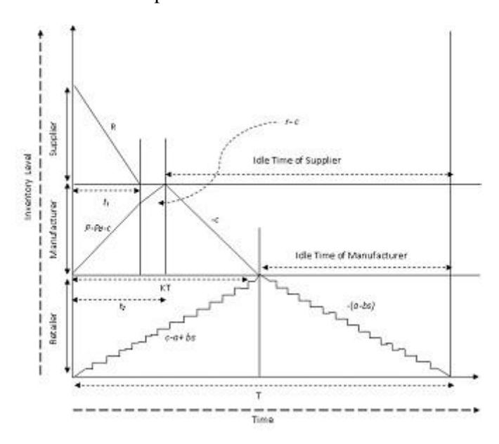
Figure 1 Three-layer inventory flow chart.
We assumed that the manufacturer produces both good and defective units of the product. Furthermore, we also assumed that the defective units of the product are all reworkable by the manufacturer and that the rework process is started after completion of regular production. We developed our three-stage supply chain model considering retailer price dependent demand with a three-level trade credit policy using the following assumptions: (1) the supplier offers a certain permissible period of payment delay to the manufacturer; (2) the manufacturer offers a certain permissible period of payment delay to the retailer, and (3) the retailer offers a permissible period of payment delay to the customers. Finally, we found out the profit function of each SCM for various credit period cases.
The objective of this research was to find the optimal selling price per unit for the retailer's optimum production rate P per unit time for manufacture, and the optimum cycle time T for various credit time intervals with respect to two different coordination policies. The first one is a collaborative (integrated) and the second one is a Stackelberg leadership policy. Finally, we analyzed which coordination policy is better than the other and also determined which credit scheme is the most favorable for each SCM.
2 Notations and Assumptions
The following notations are used in this model:
R = Lot size of replenishment at the supplier's level,
P = Manufacturing rate of the manufacturer, which is equal to the replenishment rate provided by the supplier to the manufacturer, and it is also equal to their work rate to produce good items from defective items.
\(h_s\) = Inventory holding cost per unit time for the supplier,
\(h_m\) = Inventory holding cost of good items per unit time for the manufacturer,
\(h_r\) = Inventory holding cost per unit time for the retailer, c = Demand rate of the retailer from the manufacturer,
\(D_c(s)\) = Demand rate of the customers from the retailer, where \(D_c(s)\) = (a - bs) and \(c > D_c(s)\), s = Selling price of product per unit at the retailer's level,
\(w_s\) = Wholesale price of the product (in package form) at the supplier's level, n = Number of units of the finished product at the manufacturer's level, which is equal to \(\frac{1}{n}\) time of a single unit of raw material,
\(\mu\) = Rework cost per unit of product for the manufacturer,
\(w_m\) = Wholesale price per unit of product at the manufacturer's level,
\(A_s\) = Setup cost per order for the supplier,
\(A_r\) = Setup cost per order for the retailer,
\(A_m\) = Setup cost per order for the manufacturer, m = Permissible period of payment delay offered by the manufacturer to the retailer.
Permissible period of payment delay offered by the retailer to the customers,
\(P_d\) = Defective items production rate per unit time,
\(I_m\) = Per unit idle time cost of the manufacturer,
\(I_s\) = Per unit idle time cost of the supplier,
E(x) = Expected value of variable x,
\(I_c\) = Interest rate per unit $ payable by the manufacturer and the retailer,
= Interest rate per unit $ earned by the manufacturer and the retailer,
= Expected net profit of the manufacturer, where = 1,2,3,4,
= Expected integrated net profit of the supply chain, where = 1,2,3,4,
= Net profit of the manufacturer, where = 1,2,3,4,
= Net profit of the supplier, where = 1,2,3,4,
= Net profit of the retailer, where = 1,2,3,4, 1 = Regular production run time of the product,
= Rework time for production of good items from defective items, where = 2−1,, 2 = Sum of regular production time and rework time,
= Screening cost per unit product,
= Purchasing cost per unit product of the supplier (in package form), ℎ = Holding cost of defective items, ℎ = Holding cost of reworkable items.
2.1 Assumptions
The following assumptions were used in the model:
- 1. Regular production and rework rate per unit time are equal,
- 2. Defective items are fully converted into good items and no items are scrapped,
- 3. Customer demand rate Dc(s) = (a-bs) is price sensitive, where b is a price sensitive coefficient of price, and a is the base demand rate of the customers and c > Dc(s),
- 4. During the rework process machine breakdown probability is the same as during the regular production process,
- 5. Fixed replenishment rate, production rate P and selling price s are the decision variables,
- 6. Holding costs are constant,
- 7. Production of defective items follows a probability distribution at manufacturer's level,
- 8. Stock-out situation is neglected,
- 9. Lead time is zero,
- 10. Credit coordination policy is made only for ≤ 1,
- 11. The supplier's supplying capacity is infinite,
- 12. The production capacity of the manufacturer is sufficiently large as compared to product demand.
3 Mathematical Model
In this section, we present three-level trade credit supply chain production system, which includes two vertical marketing strategies. In the first strategy, we consider the supplier, the manufacturer and the retailer working together in a collaborative (integrated) environment. In the second strategy, we consider the supplier, the manufacturer and the retailer working together in a Stackelberg leadership environment, where the manufacturer acts as the leader of the SCN and the others are followers. The profit functions of the SCMs are as follows.
3.1 The Model for Collaborative Environment
3.1.1 Supplier's Profit Function
The supplier supplies the raw material of the product to the manufacturer continuously in time interval \([0, t_I]\) to meet the production demand of the manufacturer. If P is the production rate of the product per unit time, then at time t, the inventory level of the supplier is governed by the following differential equation:
\[\frac{dI_s}{dt} = -P \tag{1}\]
With boundary conditions at t=0, \(I_s(0)=q\) and \(I_s(t_1)=0\), \(0 \le t \le t_1\), Eq. (1) leads to:
\[I_s(t) = -Pt + A, 0 \le t \le t_1, \text{ again } I_s(t_1) = 0, t_1 = \frac{R}{P}\] (2)
Now, the profit function of the supplier can be formulated as:
total revenue = \(w_s R\), setup cost = \(A_s\), cost of ideal time = \(I_s(T - t_1)\), purchasing cost =\(c_s R\), inventory holding cost = \(h_s \int_0^{t_1} (R - Pt_1) dt = \frac{1}{2} h_s Pt_1^2\), screening cost = \(S_c R\).
Then, the profit of the supplier is:
\[PS = w_s P t_1 - s_c P t_1 - A_s - c_s P t_1 - I_s (T - t_1) - \frac{1}{2} h_s P t_1^2\] (3)
3.1.2 Manufacturer's Profit Function
After receiving the raw material from the supplier, the manufacturer produces perfect and imperfect products in time interval \([0, t_I]\). After that time interval, the manufacturer stops production and in time interval \([t_1, t_2]\) he starts the rework process on defective units. If P is the regular production rate per unit time, \(P_d\) is the defective item production rate per unit time, and c is the demand rate per unit
time of the product from the retailer's end. Then, at time t, the following differential equation represents the manufacturer's inventory level for the four different intervals:
\[\frac{dI_{m_1}(t)}{dt} = P - P_d - c,\tag{4}\] with the conditions at 1 (0) = 0 and 1 (1 ) = 1, 0 ≤ ≤ 1.
Eq. (4) leads to
\[I_{m_1}(t_1) = (P - P_d - c)t_1 = z_1, 0 \le t \le t_1\] (5)
In the interval (t1, t2), the inventory status is governed by the following differential equation:
\[\frac{dI_{m_2}(t)}{dt} = r - c \tag{6}\] with the conditions 2 (0) = 1, 1 ≤ ≤ 2.
By using the boundary conditions, Eq. (6) leads to:
\[I_{m_2}(t) = (r - c)t + z_1, t_1 \le t \le t_2 \text{ and}\] \[I_{m_2}(t) = (r - c)t + (p - P_d - r)t_1, t_1 \le t \le t_2\] (7)
In the interval (2,), the inventory status is governed by the following differential equation:
\[\frac{dI_{m_3}}{dt} = -c, (8)\] with boundary conditions at = ,3 () = 0, 2 ≤ ≤
\[I_{m_3}(t) = c(KT - t), t_2 \le t \le KT\] (9)
and = 2 the Eqs. (7) and (9) should be equal and assuming the rework rate is equal to the production rate, we obtain:
\[KT = \frac{Pt_1}{c} \tag{10}\]
The inventory level of defective items in the interval 0 ≤ ≤ 1 is governed by:
\[\frac{dI_d}{dt} = P_{d,} \tag{11}\] with the boundary conditions (0) = 0 and (1 ) = 1.
Then the solution is:
\[I_d(t_1) = P_d t, (12)\]
The inventory level of defective items that are reworked in the interval \(t_1 \le t \le t_2\) is governed by:
\[\frac{dI_r}{dt} = -P,\tag{13}\] with the boundary conditions \(I_d(t_1) = Pt_1x\) and \(I_d(t_2) = 0\). Then the solution is:
\[I_r(t) = P(t_2 - t) \tag{14}\]
Now, the profit function of the manufacturer can be formulated as: Revenue from sales = \(nw_mPt_1\), production cost per unit of finished product
\[PC = w_s + \frac{\Gamma}{P} + \gamma P\], (as in Pal et al. [34]).
The total production cost in the period \([0, t_1]\) is \(TPC = PC = (w_s + \frac{\Gamma}{P} + \gamma P)Pt_1\), the rework cost for defective items is \(RC = \mu Pxt_1\), setup cost. Idle = \(A_m\), idle time cost = \(I_m(T - KT)\), and the inventory holding cost is:
IHC = \[h_m \left[ \int_0^{t_1} (P - c) t dt + \int_{t_1}^{t_2} (r - c) t dt + \int_{t_2}^{KT} c(KT - t) dt \right]\]
The inventory holding cost of defective items is (using Eq. (12)):
\[IHC_d = h_{cd} \int_0^{t_2} I_d(t_1) dt = h_{cd} \int_0^{t_2} P_d t dt = \frac{1}{2} P_d h_{cd} t_1^2 = \frac{1}{2} h_{cd} P t_1^2 x \quad (15)\]
The inventory holding cost of defective items that are reworked during the interval \(t_1 \le t \le t_2\) (from Eq. (14)) is:
\[IHC_r = h_{cr} \int_{t_1}^{t_2} I_d(t) dt = h_{cr} \int_{t_1}^{t_2} P(t_2 - t) dt = \frac{1}{2} h_{cr} P t_1^2 x^2\] (16)
The net profit function for the manufacturer is:
\[PM = nw_m Pt_1 - (w_s + \frac{\Gamma}{P} + \gamma P)Pt_1 - \mu Pxt_1 A_m - I_m (T - KT) - h_m \left[ \frac{Pt_2^2}{2} + \frac{cK^2T^2}{2} - cKTt_2 \right] - \frac{1}{2}h_{cd}Pt_1^2x - h_{cr}Pt_1^2x^2,\] (17)
where \(\tau = t_2 - t_1\), is the rework time for the manufacturer to produce good items from defective items.
3.1.3 Retailer's Profit Function
During time interval [0, KT], the retailer receives the good units of the product from the manufacturer and sells the product to customers simultaneously. After that time interval, he stops receiving the product and only continues the sales in the remaining time interval [KT, T]. If c per unit time is the retailer's demand rate, and \(D_c(s) = (a - bs)\) per unit time is the customers' demand rate, then for two various intervals the retailer's inventory level can be represented by the following differential equations:
\[\frac{dI_{r_1}(t)}{dt} = (c - D_c(s)),\tag{18}\] with the boundary conditions at t = 0, \(I_{r_1}(0) = 0\), \(0 \le t \le KT\), where \(D_c(s) = (a - bs)\).
For the interval (KT, T), the inventory status is governed by the following DE:
\[\frac{dI_{r_2}(t)}{dt} = D_c(s),\tag{19}\] with initial conditions at t = T, \(I_{r_2}(T) = 0\), \(KT \le t \le T\).
Using the initial condition \(I_{r_1}(t) = (c - D_c(s))t\) and \(I_{r_2}(t) = D_c(s)(T - t)\) and at t = KT, \(I_{r_1}(t) = I_{r_2}(t)\) i.e., \((c - D_c(s))KT = D_c(s)(T - KT)\), then \(K = \frac{D_c(s)}{c} < 1\) (according to assumption 2).
As we have assumed \(c > D_c(s)\), it is a requirement for model stability for the time interval follows the condition \(t_1 < KT < T\).
Now, the profit function of the supplier can be formulated as follows: revenue from sales = \((w_r - w_m)D_c(s)T\), setup cost = \(A_r\), inventory holding cost
\[IHC_r = h_r \left[ \int_0^{KT} (c - D_c(s)) t dt + \int_{KT}^T D_c(s) (KT - t) dt \right]\] (22)
For the net profit function of the retailer (using Eqs. (10) and (22)) we get:
\[PR = (w_r - w_m)Pt_1 - A_r - h_r \left[ \frac{3P^2t_1^2}{2c} - D_c(s) \frac{P^2t_1^2}{c^2} - \frac{P^2t_1^2}{2D_c(s)} \right]\](23)
3.1.4 Various Cases for Trade Credit Policy
According to the assumptions, if the manufacturer accepts the supplier's permissible payment delay period l at time t=0, and the manufacturer provides permissible payment delay period m to the retailer and the retailer provides permissible delay period of payment n to his customers, then after the end of the prescribed periods the manufacturer, the retailer and the customers start to pay their basic dues along with interest in installments, because they are unable to pay all dues instantly. We developed four cases with various permissible payment delay periods. Within time interval \([0, t_1]\) these are:
- (i) ≤ ≤ ≤ 1
- (ii) ≤ ≤ ≤ 1
- (iii) ≤ ≤ ≤ 1
- (iv) ≤ ≤ ≤ 1
We applied these respective cases one by one to the profit function for optimization.
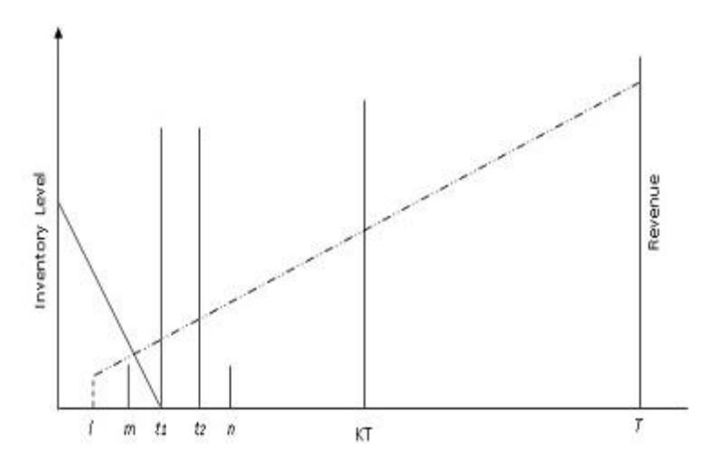
Figure 2 Revenue collection graph of supplier, Case 1.
3.1.5 Case 1: If ≤ ≤ ≤
According to the restrictions of this case, the manufacturer pays interest to the supplier along with the basic dues. Similarly, the retailer also pays interest to the manufacturer along with the basic dues. Obviously, after the end of the credit period, the manufacturer and the retailer are both unable to pay all their dues to the supplier and the manufacturer, respectively, because they are not able to sell all the products within the credit period and so they bear interest. Revenue collection, interest payment, and inventory level graphs of the supplier, manufacturer and retailer respectively are given in Figures 2-4.
3.1.6 Evaluation of Earned/Paid Interest for Supply Chain Members
Due to the restrictions on the various credit periods offered/permitted by the SCMs and the variability of the inventory level in various sub intervals, the respective paid/earned interest amounts of the manufacturer and the retailer may be formulated as follows:
(i) Interest paid by the manufacturer to the supplier in the finite time horizon T is:
\[IS_{m} = w_{s}I_{c} \left[ \int_{l}^{m} Ptdt + \int_{m}^{t_{1}} (P - D_{c}(s))tdt + \int_{t_{1}}^{\tau} (Pt_{1} - D_{c}(s)t)dt \right]\](24)
(ii) Interest paid by the retailer to the manufacturer in the finite time horizon T is:
horizon T is:
\[IS_r = w_m I_c \left[ \int_m^n ct dt + \int_n^{KT} (c - D_c(s)t) dt + \int_{KT}^T (cKT - D_c(s)t) dt \right]\]
(25)
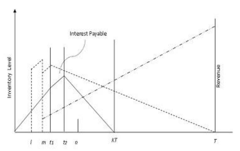
Figure 3 Revenue and interest payment graph of the manufacturer, Case 1.
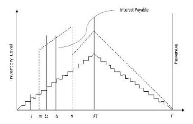
Figure 4 Revenue collection graph of the retailer, Case 1.
3.1.7 Expected Integrated Net Profit of Supply Chain
Including the coordination policy of this case, the respective individual net profits of the supplier, the manufacturer, and the retailer are:
\[NPS_1 = PS, NPM_1 = PM - IS_{ml}, NPR_1 = PR - IS_{rl}\] where PS, PM, PR, \(IS_{ml}\) and \(IS_{rl}\) are given by Eqs. (3), (17), (23), (24) and (25), respectively, and the integrated net profit function of the whole supply chain is:
\[INP(P,s) = PS + PM - IS_{ml} + PR - IS_{rl}\] (26)
and hence the expected integrated net profit of the whole supply chain is:
\[EINP_1(P,s) = EINPS_1(P,s) + EINPM_1(P,s) + EINPR_1(P,s),\]
To simplify, if we use the notation \(\Pi_{ij}^c\), where i=0,1,2,3,4,5,6 indexing for the different coefficients of the combination of variables P,s,j=1,2,3,4 indexing for the different cases, where \(\mathbf{c}\) denotes the coordination policy, then
\[ENIP_{1}(P,s) = \Pi_{01}^{c} + \Pi_{11}^{c}P - \Pi_{21}^{c}P^{2} - \Pi_{31}^{c}D_{c}(s) + \Pi_{41}^{c}D_{c}(s)P^{2} - \Pi_{51}^{c}PD_{c}(s)^{-1} - \Pi_{61}^{c}P^{2}D_{c}(s)^{-1}\](27)
where \[\Pi_{01}^{c} = I_{s}t_{1} - A_{s} - \Gamma t_{1} - A_{m} - A_{r} + \frac{1}{2}w_{m}I_{c}cm^{2}\],
\[\begin{split} \Pi_{11}^{c} &= (\mathbf{w}_{s} - \mathbf{c}_{s} - \mathbf{s}_{c})\mathbf{t}_{1} - \frac{1}{2}\mathbf{h}_{r}\mathbf{t}_{1}^{2} + \mathbf{a}\mathbf{w}_{m}\mathbf{t}_{1} - \mathbf{w}_{s}\mathbf{t}_{1} - \frac{1}{2}h_{m}t_{1}^{2}E(x^{2}) + \frac{1}{2}h_{m}t_{1}^{2} \\ &- h_{cd}t_{1}^{2}E(x) - h_{cr}t_{1}^{2}E(x^{2}) - \mu t_{1}E(x) + \frac{I_{m}t_{1}}{c} \\ &+ \frac{1}{2}\mathbf{w}_{s}I_{c}(t_{1}^{2} + \mathbf{l}^{2}) + (\mathbf{w}_{r} - \mathbf{w}_{m})\mathbf{t}_{1}, \end{split}\]
\[\Pi_{21}^{c} = \gamma t_{1} + \frac{I_{m}t_{1}^{2}}{2c} + \frac{3t_{1}^{2}h_{r}}{2c} - \frac{w_{m}I_{c}t_{1}^{2}}{2c},\] \[\Pi_{31}^{c} = \frac{1}{2}I_{c}(w_{s}m^{2} + w_{m}n^{2}),\] \[\Pi_{41}^{c} = \frac{h_{r}t_{1}^{2}}{c^{2}},\]
\[\Pi_{51}^{c} = (I_s + I_m)t_1, \Pi_{61}^{c} = (w_sI_c + w_mI_c - h_r)\frac{t_1^2}{2}.\]
3.1.8 Case 2: If \(l \le n \le m \le t_1\)
According to the restrictions of this case, the retailer earns interest along with the sales revenue during the time interval from n to m from the customers. The retailer is also unable to pay all the dues of the manufacturer within time period m, because he is not able to sell all the units of the product in that period, so he
accepts the interest due over the time period from m to T. Similarly, the manufacturer also pays interest and basic dues after the end of credit period l, because he is not able to sell all units of the product within time period l, so he bears the interest and basic dues during the time period from m to T. Revenue collection, interest payment and inventory level graphs of the supplier, manufacturer and retailer, are given in Figures 5 and 6, respectively.
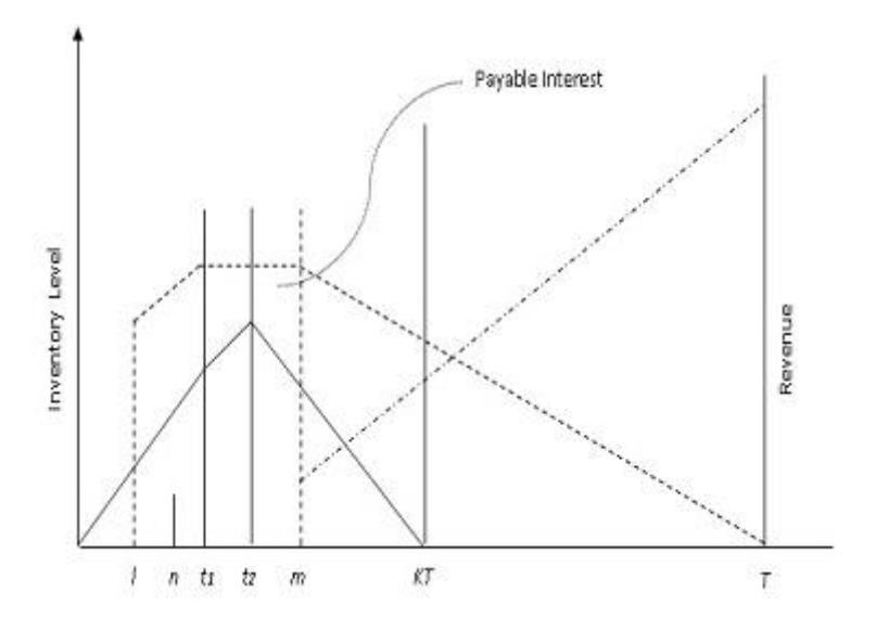
Figure 5 Revenue collection graph of the manufacturer, Case 2.
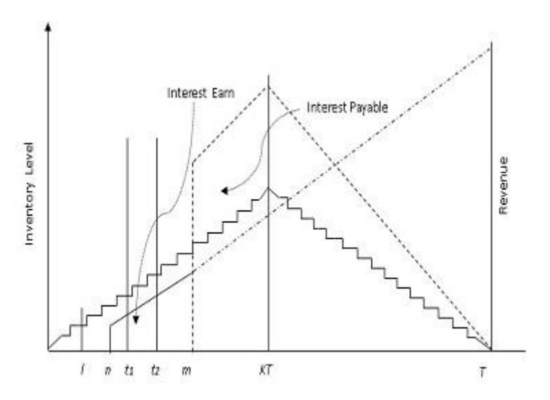
Figure 6 Revenue collection graph of the retailer, Case 2.
3.1.9 Evaluation of Earned/Paid Interest for Supply Chain Members
According to the restrictions on the credit periods offered/permitted by the SCMs and the variability of the inventory level in the various sub intervals, the respective paid/earn interest amounts for the manufacturer, the retailer, and the customers may be formulated as follows:
(i) The interest paid by the manufacturer to the supplier in the finite time horizon T is:
\[IS_{m_2} = w_s I_c \left[ \int_l^{t_1} Pt dt + \int_{t_1}^m P dt + \int_m^T (Pt_1 - D_c(s)t) dt \right].\] (28)
(ii) The interest paid by the retailer to the manufacturer in the finite time horizon T is:
\[IS_{r2} = w_m I_c \left[ \int_m^{KT} (c - D_c(s)) t dt + \int_{KT}^T ((c - D_c(s)) KT - D_c(s) t) dt \right].\] (29)
(iii)The interest earned by the retailer from the customers according to the situation is:
\[IG_{r_2} = w_r I_e \left[ \int_n^m (a - bs)t dt \right]. \tag{30}\]
Including the earned/paid interest for the supply chain members in this case, the individual net profits of the supplier, the manufacturer, and the retailer are respectively:
\[NPS_2 = PS, NPM_2 = PM - IS_{m_2}, NPR_2 = PR - IS_{r_2} + IG_{r_2}\] where PS, PM, PR, \(IS_{m_2}\), \(IS_{r_2}\) and \(IG_{r_2}\) are given by Eqs. (3), (17), (23), (24), (28)-(30), respectively, and the integrated profit function of the whole supply chain is:
\[INP(P,s) = PS + PM - IS_{m_2} + PR - IS_{r_2} + IG_{r_2}\] (31)
and hence the expected net integrated net profit of the whole supply chain is:
\[EINP_{2}(P,s) = EINPS_{2}(P,s) + EINPM_{2}(P,s) + EINPR_{2}(P,s)\](32)
\[ENIP_{2}(P,s) = \Pi_{02}^{c} + \Pi_{12}^{c}P - \Pi_{22}P^{2} - \Pi_{32}^{c}D_{c}(s) + \Pi_{42}D_{c}(s)P^{2} - \Pi_{52}^{c}PD_{c}(s)^{-1} - \Pi_{62}^{c}P^{2}D_{c}(s)^{-1}\] where \[\Pi_{02}^{c} = I_{s}t_{1} - A_{s} - \Gamma t_{1} - A_{m} - A_{r} + \frac{1}{2}w_{m}I_{c}cm^{2}\],
\[\begin{split} \Pi_{12}^{c} &= (w_{s} - c_{s} - s_{c})t_{1} - \frac{1}{2}h_{r}t_{1}^{2} + aw_{m}t_{1} - w_{s}t_{1} - \frac{1}{2}h_{m}t_{1}^{2}E(x^{2}) + \frac{1}{2}h_{m}t_{1}^{2}\\ &- h_{cd}t_{1}^{2}E(x) - h_{cr}t_{1}^{2}E(x^{2}) - \mu t_{1}E(x) + \frac{I_{m}t_{1}}{c}\\ &+ \frac{1}{2}w_{s}I_{c}(t_{1}^{2} + l^{2}) + (w_{r} - w_{m})t_{1},\\ \Pi_{22}^{c} &= \gamma t_{1} + \frac{h_{m}t_{1}^{2}}{2c} + \frac{3t_{1}^{2}h_{r}}{2c} - \frac{3w_{m}I_{c}t_{1}^{2}}{2c},\\ \Pi_{32}^{c} &= \frac{1}{2}(w_{s}m^{2}I_{c} + w_{m}n^{2}I_{c} - w_{r}I_{e}(m^{2} - n^{2})),\\ \Pi_{42}^{c} &= \frac{h_{r}t_{1}^{2}}{c^{2}} - \frac{w_{m}I_{c}t_{1}^{2}}{c^{2}},\\ \Pi_{52}^{c} &= (I_{s} + I_{m})t_{1},\\ \Pi_{62}^{c} &= (w_{s}I_{c} + w_{m}I_{c} - h_{r})\frac{t_{1}^{2}}{2}. \end{split}\]
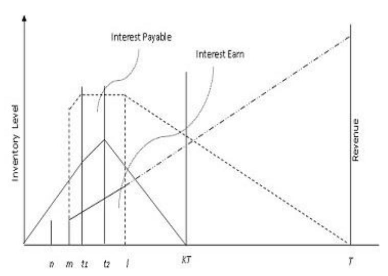
Figure 7 Revenue collection of the manufacturer, Case 3.
3.1.10 Case 3: If \(n \le m \le l \le t_1\)
According to the restrictions on the credit periods in this case, the manufacturer and the retailer both earn interest at rate \(I_e\) per unit of the product along with the sales revenue. After the end of credit period l, the manufacturer starts to pay the interest along with the basic dues. Until this time, the manufacturer is unable to pay all basic dues, as the sale of all units of the product is not complete until time l, therefore he bears interest up to time T. Similarly, after the end of credit period m, the retailer starts to pay interest along with the basic dues. Until this time, the retailer is also unable to pay all basic dues, as his sale of all units of the product is not complete until time m, therefore he bears interest up to time T. Revenue collection, interest payment, and inventory level graphs of the manufacturer and retailer respectively are given in the Figures 7 and 8.
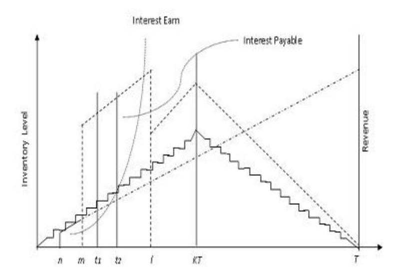
Figure 8 Revenue collection of the manufacturer, Case 3.
3.1.11 Evaluation of Earned/Paid Interest for Supply Chain Members
According to the restrictions on the credit periods offered/permitted by the SCMs and the variability of the inventory level in the various sub intervals, the paid/earn interest amounts for the manufacturer, the retailer and the customers respectively may be formulated as follows:
(i) The interest paid by the manufacturer to the supplier in the finite time horizon T is:
\[IS_{m_3} = w_s I_c \left[ \int_m^{t_1} Pt dt + \int_{t_1}^l Pt_1 dt + \int_l^T (Pt_1 - D_c(s)t) dt \right]. \tag{33}\]
(ii) The interest paid by the retailer to the manufacturer in the finite time horizon T is:
\[IS_{r_{3}} = w_{m}I_{c} \left[ \int_{m}^{KT} (c - (D_{c}(s))tdt + \int_{KT}^{T} (cKT - D_{c}(s)t)dt \right]. (34)\]
(iii) The interests gained by the manufacturer and the retailer are respectively:
\[IG_{m_3} = w_m I_e \int_m^l ct dt, IG_{m_3} = w_r I_e \left[ \int_n^m (a - bs) t dt \right]\] (35)
Including the earned/paid interest of the SCMs in this case, the individual net profits of the supplier, manufacturer and retailer are respectively:
\[NPS_3 = PS, NPM_3 = PM - IS_{m_3} + IG_{m_3}, NPR_3 = PR - IS_{r_3} + IG_{r_3}\] where PS, PM, PR, \(IG_{m_3}\), \(IG_{r_3}\), \(IS_{m_3}\) and \(IS_{r_3}\) are given by Eqs. (3), (17), (25), and (33)-(35), respectively, and the integrated net profit function of the whole supply chain is:
\[INP(P,s) = PS + PM + IG_{m_3} - IS_{m_3} + PR + IG_{r_3} - IS_{r_3}\] (36)
and hence the expected net integrated net profit of the whole supply chain is:
\[ENIP_{3}(P,s) = ENPS_{3}(P,s) + ENPM_{3}(P,s) + ENPR_{3}(P,s)\] \[ENIP_{3}(P,s) = \Pi_{03}^{c} + \Pi_{13}^{c}P - \Pi_{23}P^{2} - \Pi_{33}^{c}D_{c}(s) + \Pi_{43}D_{c}(s)P^{2}\] \[- \Pi_{53}^{c}P(D_{c}(s))^{-1} - \Pi_{63}^{c}P^{2}(D_{c}(s))^{-1},\] (37)
where
\[\begin{split} \Pi_{03}^{c} &= I_{s}t_{1} - A_{s} - \Gamma t_{1} - A_{m} - A_{r} + \frac{1}{2}w_{m}I_{c}cm^{2} + \frac{1}{2}w_{m}I_{c}c(l^{2} - m^{2}), \\ \Pi_{13}^{c} &= (w_{s} - c_{s} - s_{c})t_{1} - \frac{1}{2}h_{r}t_{1}^{2} + aw_{m}t_{1} - w_{s}t_{1} - \frac{1}{2}h_{m}t_{1}^{2}E(x^{2}) + \\ &\quad \frac{1}{2}h_{m}t_{1}^{2} - h_{cd}t_{1}^{2}E(x) - h_{cr}t_{1}^{2}E(x^{2}) - \mu t_{1}E(x) + \frac{I_{m}t_{1}}{c} + \\ &\quad \frac{1}{2}w_{s}I_{c}(t_{1}^{2} + m^{2}) + (w_{r} - w_{m})t_{1}, \\ \Pi_{23}^{c} &= \gamma t_{1} + \frac{h_{m}t_{1}^{2}}{2c} + \frac{3t_{1}^{2}h_{r}}{2c} + \frac{3w_{m}I_{c}t_{1}^{2}}{2c}, \\ \Pi_{33}^{c} &= \frac{1}{2}\Big(w_{s}l^{2}I_{c} + w_{m}m^{2}I_{c} - \frac{1}{2}w_{r}I_{e}(m^{2} - n^{2})\Big), \\ \Pi_{43}^{c} &= \frac{h_{r}t_{1}^{2}}{c^{2}}, \\ \Pi_{53}^{c} &= (I_{s} + I_{m})t_{1}, \\ \Pi_{63}^{c} &= (w_{s}I_{c} + w_{m}I_{c} - h_{r})\frac{t_{1}^{2}}{2}. \end{split}\]
3.1.12 Optimality Criteria
Proposition: The manufacturer's production rate \(P_i\) and retail price \(s_i\) have an optimal point \((P_i^*, s_i^*)\), where i = 1, 2, 3 (this is true for cases 1, 2, and 3).
Proof: Profit function \(ENIP_i(P, s)\) is optimal at point \((P_i^*, s_i^*)\), if the first order partial derivative of \(ENIP_i(P, s)\), must be vanished at point \((P_i^*, s_i^*)\), i.e.,
\[\frac{\partial ENIP_i(P_i,s_i)}{\partial P_i} = 0\] and \(\frac{\partial ENIP_i(P_i,s_i)}{\partial s_i} = 0\) at \((P_i^*, s_i^*)\), where \(i = 1, 2, 3\)
Therefore.
\[\Pi_{1i}^{c} - 2\Pi_{2i}^{c}P + 2\Pi_{4i}^{c}D_{c}(s)P - \Pi_{5i}^{c}D_{c}(s)^{-1} - 2\Pi_{6i}^{c}PD_{c}(s)^{-1} = 0\] (38)
\[\Pi_{3i}^{c}b - \Pi_{4i}^{c}bP^{2} - \Pi_{5i}^{c}Pb(D_{c}(s))^{-2} - \Pi_{6i}^{c}P^{2}b(D_{c}(s))^{-2} = 0\] (39)
Solving the above system of two equations, we have optimal values of \(P_i\) and \(s_i\), where i = 1, 2, 3.
Proposition: Profit function \(ENIP_i(P_i, s_i)\) is jointly concave for the values of \(P_i\) and \(s_i\) if:
\[\begin{split} &4[\Pi_{2i}^c-\Pi_{4i}^cD_c(s)+\Pi_{6i}^cD_c(s)^{-1}][\Pi_{5i}^cP(D_c(s))^{-3}+\\ &\Pi_{6i}^cP(D_c(s))^{-3}]-[2\Pi_{4i}^cP+\Pi_{5i}^cP(D_c(s))^{-2}+2\Pi_{6i}^cP(D_c(s))^{-2}]^2>\\ &0,), \text{where } i=1,2,3. \end{split}\]
Proof: The second order partial derivatives of \(ENIP_i(P,s)\) are:
\[\begin{split} &\frac{\partial^2 ENIP_i(P_i,s_i)}{\partial P_i^2} = -2 [\Pi_{2i}^c - \Pi_{4i}^c D_c(s) + \Pi_{6i}^c D_c(s)^{-1}], \\ &\frac{\partial^2 ENIP_i(P_i,s_i)}{\partial P_i \partial s_i} = - [2 \Pi_{4i}^c Pb + \Pi_{5i}^c b (D_c(s))^{-2} + 2 \Pi_{6i}^c Pb (D_c(s))^{-2}], \\ &\frac{\partial^2 ENIP_i(P_i,s_i)}{\partial s_i^2} = -2 b^2 [\Pi_{5i}^c P(D_c(s))^{-3} + \Pi_{6i}^c P^2 (D_c(s))^{-3}]. \end{split}\]
By using the above terms and after simplification, the joint concavity condition \(rt - s^2 > 0\) of ENIP<sub>i</sub>(P<sub>i</sub>, s<sub>i</sub>) is satisfied with respect to P<sub>i</sub>, and s<sub>i</sub>.
3.1.13 Case 4: If \(m \le n \le l \le t_1\)
According to the restrictions on the credit periods in this case, the manufacturer earns interest at rate \(I_e\) per unit of the product along with the sales revenue. After the end of credit period l, the manufacturer starts paying interest along with the basic dues. Until this time, the manufacturer is unable to pay all basic dues, as his sale of all units of the product is not complete until time l, therefore he bears interest up to time l. Similarly, after credit period l0 ends, the retailer starts to pay interest along with the basic dues. Until this time, the retailer is unable to pay the basic dues, as his sale of all units of product is not complete until time l1, therefore he bears interest up to time l2. Revenue collection, interest payment and inventory level graphs of the supplier, manufacturer, and retailer are given in the Figures 9 and 10, respectively.
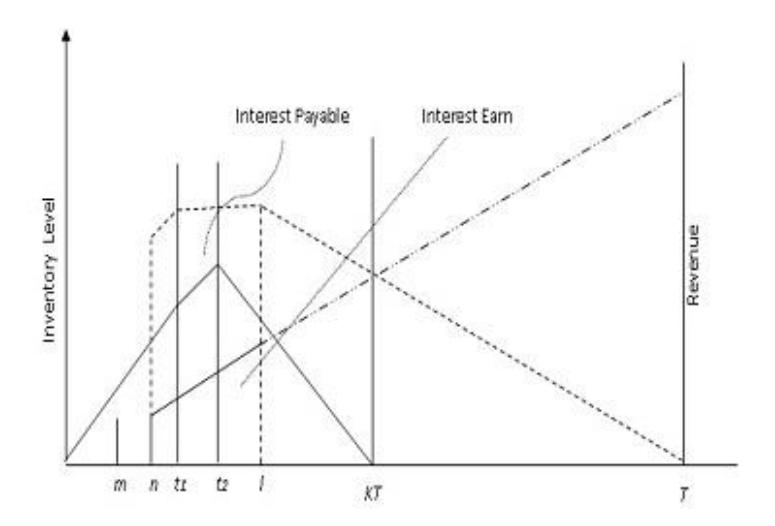
Figure 9 Revenue collection graph of the manufacturer, Case 4.
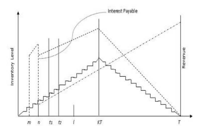
Figure 10 Revenue collection graph of the retailer, Case 4.
3.1.14 Evaluation of Earned/Paid Interest for Supply Chain Members
According to the restrictions on the credit periods offered/permitted by the SCMs and the variability of the inventory level in the various sub intervals, the paid/earned interest amount by the manufacturer, the retailer, and the customers respectively can be formulated as follows:
(i) The interest paid by the manufacturer to the supplier in the finite time horizon T is:
\[IS_{m_4} = w_s I_c \left[ \int_{l}^{m} Pt dt + \int_{m}^{t_1} (P - D_c(s)) t dt + \int_{l}^{T} (Pt_1 - D_c(s)) t dt \right]\] (40)
(ii) The interest paid by the retailer to the manufacturer in the finite time horizon T is:
\[IS_{r_{4}} = w_{m}I_{c} \left[ \int_{m}^{n} ctdt + \int_{n}^{KT} (c - (D_{c}(s)t)dt + \int_{KT}^{T} (cKT - D_{c}(s)t)dt \right]\] (41)
(iii) The interest gained by the manufacturer from the retailer is:
\[IG_{m_4} = w_m I_e \int_l^m ct dt, (42)\]
Including the paid/earned interest in this case, the individual net profits of the supplier, manufacturer and retailer are, respectively, \(NPS_4 = PS, NPM_4 = PM - IS_{m4} + IG_{m4}, NPR_4 = PR - IS_{r4}\), where PS, PM, PR, \(IG_{m4}\) and \(IS_{r4}\), are given by equations (3), (17), (25), (40), (41) and (42), respectively, and the integrated net profit function of the whole supply chain is:
\[INPS_4(P,s) = PS + PM + IG_{m_4} - IS_{m_4} + PR + IG_{r_4} - IS_{r_4}\] (43)
and hence, the expected integrated net profit of the whole supply chain is:
\[ENIP_{4}(P,s) = ENPS_{4}(P,s) + ENPM_{4}(P,s) + ENPR_{4}(P,s)\](44)
\[ENIP_{4}(P,s) = \Pi_{04}^{c} + \Pi_{14}^{c}P - \Pi_{24}P^{2} - \Pi_{34}^{c}D_{c}(s) + \Pi_{44}D_{c}(s) + \Pi_{54}^{c}D_{c}(s)P^{2} - \Pi_{64}^{c}P(D_{c}(s))^{-1} - \Pi_{74}^{c}P^{2}(D_{c}(s))^{-1},\] where
\[\begin{split} \Pi_{04}^{c} &= I_{s}t_{1} - A_{s} - \Gamma t_{1} - A_{m} - A_{r} + \frac{1}{2}w_{m}I_{c}c(n^{2} - m^{2}) + w_{m}I_{c}cn + \\ & \frac{1}{2}w_{m}I_{e}c(l^{2} - m^{2}), \\ \Pi_{14}^{c} &= (w_{s} - c_{s} - s_{c})t_{1} - \frac{1}{2}h_{r}t_{1}^{2} + aw_{m}t_{1} - w_{s}t_{1} - \frac{1}{2}h_{m}t_{1}^{2}E(x^{2}) + \\ & \frac{1}{2}h_{m}t_{1}^{2} - h_{cd}t_{1}^{2}E(x) - h_{cr}t_{1}^{2}E(x^{2}) - \mu t_{1}E(x) + \frac{I_{m}t_{1}}{c} + \\ & \frac{1}{2}w_{s}I_{c}(t_{1}^{2} + m^{2}) + (w_{r} - w_{m})t_{1} - w_{m}I_{c}t_{1}, \\ \Pi_{24}^{c} &= \gamma t_{1} + \frac{h_{m}t_{1}^{2}}{2c} + \frac{3t_{1}^{2}h_{r}}{2c} - \frac{w_{m}I_{c}t_{1}^{2}}{c}, \Pi_{34}^{c} = \frac{1}{2}w_{s}l^{2}I_{c} + \frac{1}{2}(n^{2} - m^{2} - 2n), \\ \Pi_{44}^{c} &= \frac{w_{s}I_{c}t_{1}}{c^{2}}, \Pi_{54}^{c} = \frac{h_{r}t_{1}^{2}}{c^{2}} + \frac{w_{m}I_{c}t_{1}^{2}}{2c^{2}}, \Pi_{64}^{c} = (I_{s} + I_{m})t_{1}, \end{split}\]
\[\Pi_{74}^{c} = (w_{s}I_{c} + w_{m}I_{c} - h_{r})\frac{t_{1}^{2}}{2}.\]
3.1.15 Optimality Criteria
Proposition: The manufacturer's production rate P and the retailer's retail price s have an optimal point \((P_4^*, s_4^*)\)
Proof: The same as the propositions of Subsection 3.1.12.
Proposition: Profit function \(ENIP_4(P, s)\) is jointly concave for the values of \(P_4\) and \(s_4\) if:
\[\begin{split} 4[\Pi_{24}^c - \Pi_{54}^c D_c(s) + \Pi_{74}^c D_c(s)^{-1}][\Pi_{64}^c P(D_c(s))^{-3} + \\ \Pi_{74}^c (D_c(s))^{-3} P^2] - [\Pi_{44}^c P - 2\Pi_{54}^c P - \Pi_{64}^c (D_c(s))^{-2} - \\ 2\Pi_{74}^c P(D_c(s))^{-2}]^2 > 0. \end{split}\]
Proof: The same as the propositions of Subsection 3.1.12.
3.2 Optimality Criteria when Manufacturer is Leader and Others Are Followers
Now, we consider the manufacturer as the leader and the others as followers, therefore, all decisions about the supply chain are taken by the manufacturer, so that the profits of all members are maximum. The various cases with different credit periods are as follows:
3.2.1 Case 1: If \(l \le m \le n \le t_1\)
In this case, the manufacturer's expected integrated net profit can be formulated as follows:
\[EINPM_{1} = \Pi_{01}^{s} + \Pi_{11}^{s}P - \Pi_{21}^{s}P^{2} - \Pi_{31}^{s}D_{c}(s) + \Pi_{41}^{s}P(D_{c}(s))^{-1} + \Pi_{51}^{s}P^{2}(D_{c}(s))^{-1}\] (45)
where,
\[\begin{split} \Pi_{01}^s &= -(\Gamma t_1 + A_m), \\ \Pi_{11}^s &= a w_m t_1 - w_s t_1 - \frac{1}{2} h_m t_1^2 E(x^2) + \frac{1}{2} h_m t_1^2 - h_{cd} t_1^2 E(x) - h_{cr} t_1^2 E(x^2) - \mu t_1 E(x) + \frac{l_m t_1}{c} + \frac{1}{2} w_s I_c(t_1^2 - l^2), \\ \Pi_{21}^s &= \left( \gamma t_1 + \frac{h_m t_1^2}{2c} \right), \\ \Pi_{31}^s &= \frac{1}{2} w_s I_c m^2, \end{split}\]
\[\Pi_{41}^{s} = -I_{m}t_{1},\] \[\Pi_{51}^{s} = -w_{s}I_{c}\frac{t_{1}^{2}}{2}.\]
3.2.2 Case 2: If \(l \le n \le m \le t_1\)
In this case, the manufacturer's expected integrated net profit can be formulated as follows:
\[EINPM_{2} = \Pi_{02}^{s} + \Pi_{12}^{s}P - \Pi_{22}^{s}P^{2} - \Pi_{32}^{s}D_{c}(s) + \Pi_{42}^{s}P(D_{c}(s))^{-1} + \Pi_{52}^{s}P^{2}(D_{c}(s))^{-1}\] (46)
All coefficients for this case are the same as for Case 1.
Proposition: The manufacturer's production rate P and retail price shave an optimal point \((P_i^*, s_i^*)\), where i = 1, 2.
Proof: Profit function \(ENIPM_i(P, s)\) is optimal at point \((P_i, s_i)\), if the first-order partial derivatives of \(ENIPM_i(P, s)\) must be vanished at point \((P_i^*, s_i^*)\), i.e. \(\frac{\partial ENIPM_i(P, s)}{\partial P} = 0\) and \(\frac{\partial ENIPM_i(P, s)}{\partial s} = 0\) at \((P_i^*, s_i^*)\), therefore,
\[\Pi_{1i}^{s}P - 2\Pi_{2i}^{s}P + \Pi_{4i}^{s}(D_{c}(s))^{-1} + 2\Pi_{5i}^{s}(D_{c}(s))^{-1}P = 0, \tag{47}\]
\[-\Pi_{3i}^{s}b + \Pi_{4i}^{s}(D_{c}(s))^{-2}bP + \Pi_{5i}^{c}(D_{c}(s))^{-2}bP^{2} = 0,\] (48)
where i = 1, 2. Solving the above system of two equations, we get the optimal values of \(P_i\) and \(s_i\).
Proposition: The profit function \(ENIPM_i(P, s)\) is jointly concave for the values of \(P_i\) and \(s_i\) if:
\[4\left[-\Pi_{2i}^{s} + \Pi_{5i}^{s}(D_{c}(s))^{-1}\right] \left[\Pi_{4i}^{s}(D_{c}(s))^{-3}b^{2}P + \Pi_{5i}^{s}(D_{c}(s))^{-3}P^{2}b^{2}\right] - \left[\Pi_{4i}^{s}(D_{c}(s))^{-2}b + 2\Pi_{5i}^{c}Pb(D_{c}(s))^{-2}\right]^{2} > 0, \text{ where } i = 1, 2.\]
Proof: The second order partial derivatives of \(ENIPM_i(P,s)\) are:
\[\begin{split} \frac{\partial^2 ENIPM_i(P,s)}{\partial P^2} &= 2[-\Pi_{2i}^s + \Pi_{5i}^s D_c(s)^{-1}], \\ \frac{\partial^2 ENIPM_i(P,s)}{\partial P\partial s} &= [\Pi_{4i}^s b D_c(s)^{-2} + 2\Pi_{5i}^c D_c(s)^{-2} b P], \\ \frac{\partial^2 ENIPM_i(P,s)}{\partial S^2} &= -2b^2 [\Pi_{4i}^c D_c(s)^{-3} P + \Pi_{5i}^s D_c(s)^{-3} P^2] \end{split}\] by using the above terms and after simplification, the jointly concavity condition \(rt - s^2 > 0\) of \(ENIPM_i(P, s)\) is satisfied with respect to \(P_i\) and \(s_i\).
3.2.3 Case 3: If \(n \le m \le l \le t_1\)
The manufacturer's profit function when the manufacturer is the leader, and the others are followers is:
\[EINPM_{3} = \Pi_{03}^{s} + \Pi_{13}^{s}P - \Pi_{23}^{s}P^{2} - \Pi_{33}^{s}D_{c}(s) + \Pi_{43}^{s}P(D_{c}(s))^{-1} + \Pi_{53}^{s}P^{2}(D_{c}(s))^{-1}.\] \[(49)\] \[\Pi_{03}^{s} = -\left(\Gamma t_{1} + A_{m} - \frac{1}{2}w_{m}I_{e}(l^{2} - m^{2})\right),\] \[\Pi_{13}^{s} = aw_{m}t_{1} - w_{s}t_{1} - \frac{1}{2}h_{m}t_{1}^{2}E(x^{2}) + \frac{1}{2}h_{m}t_{1}^{2} - h_{cd}t_{1}^{2}E(x) - h_{cr}t_{1}^{2}E(x^{2}) - \mu t_{1}E(x) + \frac{I_{m}t_{1}}{c} + \frac{1}{2}w_{s}I_{c}(t_{1}^{2} + m^{2}),\] \[\Pi_{23}^{s} = \left(\gamma t_{1} + \frac{h_{m}t_{1}^{2}}{2c}\right),\] \[\Pi_{33}^{s} = \frac{1}{2}w_{s}I_{c}m^{2},\] \[\Pi_{43}^{s} = -I_{m}t_{1},\] \[\Pi_{53}^{s} = -w_{s}I_{c}\frac{t_{1}^{2}}{2}.\]
3.2.4 Case 4: If \(m \le n \le l \le t_1\)
The manufacturer's profit function when the manufacturer is the leader and the others are followers is:
\[EINPM_4 = \Pi_{04}^s + \Pi_{14}^s P - \Pi_{24}^s P^2 - \Pi_{34}^s D_c(s) + \Pi_{44}^s P (D_c(s))^{-1} + \Pi_{53}^s P^2 (D_c(s))^{-1}.\] (50)
where
\[\begin{split} \Pi_{04}^s &= - \left( \Gamma t_1 + A_m - \frac{1}{2} w_m I_e(l^2 - m^2) \right) \\ \Pi_{14}^s &= a w_m t_1 - w_s t_1 - \frac{1}{2} h_m t_1^2 E(x^2) + \frac{1}{2} h_m t_1^2 - h_{cd} t_1^2 E(x) \\ &\quad - h_{cr} t_1^2 E(x^2) - \mu t_1 E(x) + \frac{I_m t_1}{c} + \frac{1}{2} w_s I_c(t_1^2 + m^2), \\ \Pi_{24}^s &= \left( \gamma t_1 + \frac{h_m t_1^2}{2c} \right), \\ \Pi_{34}^s &= \frac{1}{2} w_s I_c m^2, \\ \Pi_{44}^s &= -I_m t_1, \\ \Pi_{54}^s &= -w_s I_c \frac{t_1^2}{2}. \end{split}\]
Proposition: The manufacturer's production rate P and the retailer's retail price shave an optimal point \((P_i^*, s_i^*)\), where i = 3, 4.
Proof: The same as the proposition of Subsection 3.3.1.
Proposition: Profit function ENIPM<sub>i</sub>(P, s) is jointly concave for the values of \(P_i\) and \(s_i\) if:
\[4\left[-\Pi_{2i}^{s} + \Pi_{5i}^{s}(D_{c}(s))^{-1}\right]\left[\Pi_{4i}^{s}(D_{c}(s))^{-3}b^{2}P + \Pi_{5i}^{s}(D_{c}(s))^{-3}P^{2}b^{2}\right] - \left[\Pi_{4i}^{s}(D_{c}(s))^{-2}b + 2\Pi_{5i}^{c}Pb(D_{c}(s))^{-2}\right]^{2} > 0, \text{ where } i = 3,4.\]
Proof: The same as the propositions of Subsection 3.3.1.
3.2.5 Example 1(for Collaborative Coordination):
We considered the following dataset with parameter values:
\[a = 870, b = 0.7, c = 650, \gamma = 0.0012, w_s^c = 60, w_m = 15,\]
\(n = 10, w_r = 75, c_s = 50, s_c = 0.7, h_m = 0.8, h_r = 0.2, h_s = 0.3,\)
\(I_r = 0.02, I_m = 524, \Gamma = 5000, t_1 = 0.4, A_r = 200, A_s = 225,\)
\(A_m = 475, \circledast = 80, h_{cd} = 0.4, h_{cr} = 0.8, I_s = 225, \circledast^2 = \frac{1}{\alpha - \beta},\)
\(\alpha, \beta \in (0, 0.1), m = \frac{\alpha + \beta}{2},\)
the optimum results for the various cases are given in Table 1.
Table 1 Data table for collaborative coordination.
| Case | l | m | n | P | S | KT | T | EINPS | EINPM | EINPR | EINP | rt-s2 |
|---|---|---|---|---|---|---|---|---|---|---|---|---|
| Case | 0.1 | 0.2 | 0.3 | 1135.6 | 1142.2 | 0.86 | 7.96 | 3095 | 33839 | 31059 | 67995 | 0.00074 |
| Case 2 | 0.1 | 0.3 | 0.2 | 1341.1 | 1144.6 | 0.86 | 8.18 | 3067 | 33745 | 31154 | 67967 | 0.00071 |
| Case 3 | 0.3 | 0.2 | 0.1 | 1340.6 | 1143.9 | 0.86 | 8.18 | 3078 | 33674 | 31138 | 67890 | 0.00077 |
| Case 4 | 0.3 | 0.1 | 0.2 | 1342.4 | 1343.8 | 0.86 | 8.18 | 3084 | 33725 | 31166 | 67996 | 0.00077 |
3.2.6 Example 2 (Leader Follower Coordination):
We considered the following dataset with parameter values:
\[a = 870, b = 0.7, c = 650, \gamma = 0.0012, w_s^s = 110, w_m = 15,\]
\(n = 10, w_r = 75, c_s = 50, s_c = 0.7, h_m = 0.8, h_r = 0.2, h_s = 0.3,\)
\(I_r = 0.02, I_m = 524, \Gamma = 5000, t_1 = 0.35, A_r = 200, A_s = 225,\)
\[A_{\rm m} = 475, \ \ \oplus = 80, \ h_{\rm cd} = 0.4, \ h_{\rm cr} = 0.8, \ I_{\rm s} = 225, \ \ \ \oplus^2 = \frac{1}{\alpha - \beta},\]
\(\alpha, \beta \in (0, 0.1), \ m = \frac{\alpha + \beta}{2},\)
the optimum results for the various cases are given in Table 2.
Table 2 Data table for leader follower coordination.
| Case | l | m | n | P | s | KT | T | EINPS | EINPM EINPR | EINP | 2 rt-s | |
|---|---|---|---|---|---|---|---|---|---|---|---|---|
| Case 1 | 0.1 | 0.2 | 0.3 | 1088.9 | 1180.2 | 0.61 | 9.11 | 20361 | 39451 | 22359 | 82520 | 0.00013 |
| Case 2 | 0.1 | 0.3 | 0.2 | 1089.5 | 1177.5 | 0.61 | 8.75 | 20571 | 40082 | 22390 | 83044 | 0.00029 |
| Case 3 | 0.3 | 0.2 | 0.1 | 1089.3 | 1178.1 | 0.61 | 8.83 | 20550 | 39879 | 22378 | 80808 | 0.00026 |
| Case 4 | 0.3 | 0.1 | 0.2 | 1088.7 | 1178.1 | 0.61 | 8.82 | 20523 | 39827 | 22345 | 82697 | 0.00026 |
According to Table 3, if we fix credit period l = 0.1 permitted by the supplier and interchange the credit periods m and n permitted by the manufacturer and the retailer respectively, then the supplier's and the manufacturer's profits decrease, whereas the retailer's profit increases. Moreover, if we fix the credit period l = 0.3 and interchange the credit periods m and n permitted by the manufacturer and the retailer, respectively, then the profits of all SCMs increase.
Table 3 Sensitivity analysis for the data given in Table 1.
| l | m | n | EINPS | EINPM | EINPR |
|---|---|---|---|---|---|
| For l = 0.1 | 0.2 ↔ 0.3 | ↓ | ↓ | ↑ | |
| For l = 0.3 | 0.2 ↔ 0.1 | ↑ | ↑ | ↑ |
According to Table 4, if we fix the credit period l = 0.1 permitted by the supplier and interchange the credit periods m and n permitted by the manufacturer and the retailer, respectively, then the profits of all SCMs increase. Moreover, if we fix credit period l = 0.3 and interchange the credit periods m and n permitted by the manufacturer and the retailer, respectively, then the profits of all SCMs decrease.
Note:1. It is clear that in integrated collaborative coordination, Case 1 is the most favorable for the supplier and the manufacturer, whereas Case 4 is the most favorable for the retailer.
Note:2. It is also clear that under leader/follower coordination, Case 2 is the most favorable for all supply chain members.
Table 4 Sensitivity analysis for the data given in Table 3.
| l | m | n | EINPS | EINPM | EINPR |
|---|---|---|---|---|---|
| For l = 0.1 | 0.2 | ↔ 0.3 | ↑ | ↑ | ↑ |
| For l = 0.3 | 0.2 ↔ | 0.1 | ↓ | ↓ | ↓ |
4 Conclusion
This study developed a three-layer supply chain inventory model to determine the optimal production for the manufacturer and retail price for the retailer considering three stage trade credit policies under an imperfect production system. We assumed that after stopping regular production, the manufacturer starts rework on defective units of the product to convert them into perfect units.
In this study, different credit periods were considered between the supplier and the manufacturer, the manufacturer and the retailer, and the retailer and the customers, according to the actual market situation. We developed four different cases for fixed time intervals. The expected integrated collaborative net profit function was optimized by combining it with the profit functions of the supplier, the manufacturer, and the retailer, considering the price dependent demand of the customers.
We also optimized the expected net profit function, assuming the manufacturer as the leader and the others as followers (Stackelberg situation). According to the numerical data, the leadership approach was more profitable compared to the integrated collaborative approach when \(w_s^c > w_s^c\).
The following suggestions are beneficial for inventory managers:
- (i) Always keep l > m, n for better output of all SCMs and it is also necessary to make a revenue sharing contract between the supplier and the manufacturer in an integrated collaborative credit coordination policy.
- (ii) Always keep l < m, n for better output of all SCMs in a leadership credit period system.
- (iii) If management follows the collaborative coordination system, then always maintain the relation l > m > n for better output of all supply chain members.
- (iv) If management follows the leadership system, then always maintain the relation l < m < n for better output of all supply chain members.
- (v) In the trade credit financing scheme, the collaborative coordination system gives better output than the leadership system.
- (vi) Management should adopt a leadership credit coordination policy for better functioning of the supply chain.
Further research:
- (i) The current research may be extended in future research by considering time dependent demand or time dependent production.
- (ii) This model can be extended by incorporating batch size-dependent credit periods.
- (iii) This model can be extended by applying rework during the production period.
- (iv) This model can be extended by incorporating a stock-out situation at the retailer's end.
- (v) This model can also be extended by applying a screening process to separate out defective units of the product.
Acknowledgments
We thank the editor and the anonymous referees for their valuable and constructive comments, which led to a significant improvement of the initial paper.