
1 Introduction
Coronavirus 2019 (COVID-19) is a highly infectious disease caused by a virus. It has been circulating globally and has caused many people to lose their loved ones and relatives. The pandemic started in December 2019 in Wuhan, China and the disease was spread by people travelling for new year inside China [1]. The virus circulates during singing, coughing, sneezing, speaking, or breathing and the particles range from larger respiratory droplets to smaller aerosols [2].
Epidemiology modeling plays a critical role in early warning systems and the avoidance of outbreaks. Nonlinear differential equations are an important tool to illustrate the dynamics of infectious diseases and to evaluate control schemes to stop them. Different mathematical models have been formulated to investigate COVID-19 in various ways. Wickramaarachchi et al. [3] adopted an SEIR (susceptible, exposed, infected, and recovered) type mathematical model to
Received November 7th , 2021, Revised May 21st , 2022, Accepted for publication November 4th, 2022 Copyright © 2022 Published by ITB Institut for Research and Community Service, ISSN: 2337-5760, DOI: 10.5614/j.math.fund.sci.2022.54.2.1
outline the dynamics of COVID-19 in Sri Lanka. They focused on examining the monitoring measures against the disease's transmission and the time of implementation in the community during the epidemic's initial months. Their analysis concluded that if policymakers put up strict control measures, peaks can be delayed, and the curve can be flattened. Moshen [4] probed the global stability of a COVID-19 model with a quarantine approach together with the effect of media coverage. This may have been as a result of fear the media was spreading about the disease's reproduction number. From their analysis, they surmised that the reproduction number clearly conformed to the disease's transmission rate. Seidu [5] developed and analyzed a deterministic ordinary differential equation model for SARS-CoV-2 in view of the function of exposed, mildly symptomatic, and severe symptomatic cases in terms of the disease's transmission. Their analysis revealed that reduction of contact via the use of nasal masks and physical distancing reduces SARS-CoV-2 transmission. Alshammari [6] considered the impact of asymptomatic COVID-19 cases on the disease's spread using an altered version of a SEIR dynamical model. Analytical and numerical estimation expressions of the basic reproduction number of COVID-19 in Saudi Arabia were obtained. He et al. [7] built an SEIR epidemic model for COVID-19 based on some universal methods of regulating. They used the Particle Swarm Optimization (PSO) algorithm to get an estimate of the system's parameters and employed the developed model to show the evolution of the pandemic. Dmitry et al. [8] used simple epidemic models to forecast the spread of COVID-19 in Russia and carried out a numerical forecast according to a public data set. They also presented a comparison between SIR and SEIR models. Their models predicted the highest number of contaminated people while sustaining quarantine measures. Cooper et al. [9] investigated the effectiveness of the spread of COVID-19 within some communities using an SIR model. They investigated the time evolution of various populations and monitored varied significant parameters for the spread of the disease. They concluded that the spread could be controlled if proper measures were adhered to. Munoz-Fernandez et al. [10] showed that the official data released by several authorities concerning COVID-19 were consistent with a non-autonomous SIR model. They constructed a model whose outcome fit available real data on COVID-19. They also predicted the development of the COVID-19 pandemic in some countries. Alenezi et al. [11] carried out an analysis of COVID-19 in Kuwait using an SIR model. They investigated the impact of preventive measures taken by Kuwait's local authorities to prevent the spread of COVID-19. Their investigation indicated the peak infection rate and anticipated dates for Kuwait. Liu [12] considered latentinfectious-recovery periods and carried out an analytical solution of an SIR-like model in Excel. He concluded that the simulated epidemic curve of the model fit perfectly with daily reported cases in the region mentioned in the paper. Zhu & Shen [13] proposed a modified SIR model to investigate the spread of COVID-19 for a specified period. Their investigation revealed that the cure rate was approximately 0.05, while the reproduction number for the specified time was 0.4490.
Subrata et al. [14] proposed and analyzed an SEIR model. They studied the dynamical behavior and the stability of the model and compared the analysis of scenarios in two countries. Wintachai & Prathom [15] formulated an SEIR model that takes into account the efficiency of vaccination by forecasting the COVID-19 situation by the time vaccines were out.
Hospitalization, death, and testing data stability approximations were used by Albani et al. [25] to estimate underreported infections. Additionally, they evaluated how underreporting affected the development of vaccination plans. Daily COVID-19 reports from Chicago and New York City were used by Vinicius et al. [26] to estimate the parameters of an SEIR model that accounts for varying intensities. Impressively, their model was able to reproduce the observed data. Some other works also dealt with optimal control analysis, including [27- 29].
In this paper, we offer a mathematical model of two COVID-19 strains. A mathematical analysis was carried out in conjunction with the epidemic indicator for the proposed models, the basic reproduction number for the model was derived, and finally the model's numerical simulation was analyzed. The rest of this paper is structured as follows. The mathematical formulation of the problem is offered in Section 2. The model analysis is presented in Section 3, including the positivity solution, the boundedness of the solution, the invariant region of the model, the basic reproduction number, and equilibria. Section 4 deals with the numerical simulation, and Section 5 contains the conclusion.
2 Model Problem
It is assumed in our models that once each strain is contracted, it gives persistent immunity to itself and other strains. We use a compartmental model with six compartments. These compartments are: Susceptible (), Exposed (), Infectious strain 1 1(), Infectious strain 2 2(), Quarantine (), Recovered (). A susceptible individual, with a constant recruited rate Λ, can be infected by Strain 1 or by Strain 2 with transmission rate 1 and 2 respectively and move to the Exposed compartment. Individuals in the Exposed compartment show no symptoms and are unable to transmit the disease. After an incubation period of 5 to 14 days, individuals in the Exposed compartment become infectious at rate . A fraction of exposed individuals are fully infected by Strain 1, while the fraction of exposed individuals (1 − ) are fully infected by Strain 2 after the incubation period. The recovery rates for the two strains are 1 and 2 respectively, while 1 and 2 are the detection rates for Strains 1 and 2. is the recovery rate from the Quarantine compartment. We assume natural mortality rate \(\mu\) for individuals in all six compartments, while compartments E(t), \(I_1(t)\), \(I_2(t)\) and Q(t) have extra disease-induced death rate \(\delta\). The whole population N(t) for the dynamic transmission at any time t is given by:
\[N(t) = S(t) + E(t) + I_1(t) + I_2(t) + Q(t) + R(t)\]
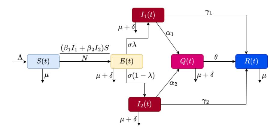
Figure 1 Compartmental diagram of disease transmission.
\[\frac{dS(t)}{dt} = \Lambda - \frac{\beta_{1}I_{1}(t)S(t)}{N} - \frac{\beta_{2}I_{2}(t)S(t)}{N} - \mu S(t) \frac{dE(t)}{dt} = \frac{\beta_{1}I_{1}(t)S(t)}{N} + \frac{\beta_{2}I_{2}(t)S(t)}{N} - (\sigma + \mu + \delta)E(t) \frac{dI_{1}(t)}{dt} = \lambda \sigma E(t) - (\gamma_{1} + \alpha_{1} + \mu + \delta)I_{1}(t) \frac{dI_{2}(t)}{dt} = (1 - \lambda)\sigma E(t) - (\gamma_{2} + \alpha_{2} + \mu + \delta)I_{2}(t) \frac{dQ(t)}{dt} = \alpha_{1}I_{1}(t) + \alpha_{2}I_{2}(t) - (\theta + \mu + \delta)Q(t) \frac{dR(t)}{dt} = \gamma_{1}I_{1}(t) + \gamma_{2}I_{2}(t) + \theta Q(t) - \mu RR(t)\] (1)
with initial conditions
\[S(0) = S_0, E(0) = E_0, I_1(0) = I_{01}, I_2(0) = I_{02}, Q(0) = Q_0, R(0) = R_0.\]
The first four equations of (1) are independent of R(t). We consider the subsystem and carry out an analysis on it.
\[\frac{dS(t)}{dt} = \Lambda - \frac{\beta_{1}I_{1}(t)S(t)}{N} - \frac{\beta_{2}I_{2}(t)S(t)}{N} - \mu S(t) \frac{dE(t)}{dt} = \frac{\beta_{1}I_{1}(t)S(t)}{N} + \frac{\beta_{2}I_{2}(t)S(t)}{N} - (\sigma + \mu + \delta)E(t) \frac{dI_{1}(t)}{dt} = \lambda \sigma E(t) - (\gamma_{1} + \alpha_{1} + \mu + \delta)I_{1}(t) \frac{dI_{2}(t)}{dt} = (1 - \lambda)\sigma E(t) - (\gamma_{2} + \alpha_{2} + \mu + \delta)I_{2}(t) \frac{dQ(t)}{dt} = \alpha_{1}I_{1}(t) + \alpha_{2}I_{2}(t) - (\theta + \mu + \delta)Q(t)\] (2)
with initial conditions
\[S(0) = S_0, E(0) = E_0, I_1(0) = I_{01}, I_2(0) = I_{02}, Q(0) = Q_0.\]
3 Model Analysis
In this section, we carry out a quantitative study of the two-strain model, including the positivity of the solution, the boundedness of the solution, the invariant region of the model, the basic reproduction number, equilibria, and the global stability of the model.
3.1 Positivity Solution
Theorem 1: The solutions (), (),1 (),2 (),() of Equation (2) with positive initial condition are non-negative for all > 0.
Proof: We will use the first equation in Equation (2) to show the positivity of the solutions.
Let
\[T = Sup\{t > 0: S(t) > 0, E(t) > 0, I_1(t) > 0, I_2(t) > 0, Q(t) > 0\}\]
\(\in [0, t].\)
For > 0, then
\[\frac{dS(t)}{dt} = \Lambda - \left(\frac{\beta_1 I_1(t) + \beta_2 I_2(t)}{N} + \mu\right) S(t)\] \[\frac{dS(t)}{dt} = \Lambda - (k(t) + \mu) S(t)\] where \[k(t) = \frac{\beta_1 I_1(t) + \beta_2 I_2(t)}{N}\]
\[\frac{dS(t)}{dt} + (k(t) + \mu)S(t) = \Lambda\] with integrating factor, we have:
\[\frac{d}{dt}\left(S(t)exp\left\{\mu t + \int_0^t k(p)dp\right\}\right) = \Lambda exp\left\{\mu t + \int_0^t k(p)dp\right\}\]
Solving and integrating both sides from 0 to T, we have:
\[S(T) = S(0) * exp \left\{ -\left(\mu t + \int_0^T k(p)dp\right) \right\} + exp \left\{ -\left(\mu t + \int_0^T k(p)dp\right) \right\} * \left[ \int_0^T \Lambda * exp \left\{ \mu t + \int_0^t k(p)dp \right\} dt \right] > 0.\] (3)
From the result, we can see that S(t) is strictly greater than zero. With the same argument, we can also prove that E(t), \(I_1(t)\), \(I_2(t)\) and Q(t) are all strictly greater than zero.
3.2 Boundedness of the Solution
Theorem 2: All solutions of Model (1) are bounded if \(\lim_{t\to\infty} Sup\ N(t) \le \frac{\Lambda}{\mu}\), then: \(N(t) = E(t) + S(t) + Q(t) + R(t) + I_1(t) + I_2(t)\).
Proof: Let
\[\mathbf{0} < E(t) + Q(t) + R(t) + I_1(t) + I_2(t) \le N(t) \tag{4}\]
Add up all the equations in Model (1), we have:
\[\frac{dN(t)}{dt} = \Lambda - \mu N(t) - \delta \left( E(t) + Q(t) + R(t) + I_1(t) + I_2(t) \right) \tag{5}\]
Using Eq. (4) in Eq. (5), we obtain:
\[\Lambda - \delta N(t) - \mu N(t) \le \frac{dN(t)}{dt} \le -\mu N(t) + \Lambda\]
It follows from this that the solutions of the proposed Model (1) are bounded and can be written as:
\[\frac{\Lambda}{\mu + \delta} \le \lim_{t \to \infty} \inf N(t) \le \lim_{t \to \infty} \sup N(t) \le \frac{\Lambda}{\mu}.\] (6)
3.3 Invariant Region of the Model
The parameters of the models are positive for all t > 0, for a biological region. The analysis of Model (1) will be in a meaningful biological region.
Lemma 1: The closed set \(\Omega\), defined by:
\(\Omega = \left\{ \left( E(t) + S(t) + Q(t) + R(t) + I_1(t) + I_2(t) \right) \in \mathbb{R}_+^6 : N(t) \le \frac{\Lambda}{\mu + \delta} \right\}, \text{ is positive invariant for Model (1).}\)
Proof: Let
\[\begin{split} N(t) &= E(t) + S(t) + Q(t) + R(t) + I_1(t) + I_2(t) \\ \frac{dN(t)}{dt} &= \frac{d}{dt} \Big( E(t) + S(t) + Q(t) + R(t) + I_1(t) + I_2(t) \Big) \\ \frac{dN(t)}{dt} &= \Lambda - \mu N(t) - \delta \Big( E(t) + Q(t) + R(t) + I_1(t) + I_2(t) \Big) \\ \frac{dN(t)}{dt} &= \Lambda - (\delta + \mu) N(t) \end{split}\]
After solving, we have:
\[N(t) = \frac{\Lambda}{\delta + \mu} + N_0 e^{-(\delta + \mu)}, where N(0) = N_0 > 0\]
\[\lim_{t \to \infty} N(t) = \frac{\Lambda}{\delta + \mu} < N(t).\]
Hence, we conclude that \(\Omega\) is the positivity invariant for Model (1). Because of this, we can conclude that the solutions \((E(t), S(t), Q(t), R(t), I_1(t), I_2(t))\) tend to \(\Omega\).
3.4 The Basic Reproduction Number and its Associated Equilibria
3.4.1 The Basic Reproduction Number
Adopting the approach of Van den Driessche and Watmought [20-21], and utilizing the matrix of the next generation, we calculate the basic reproduction number in the following order. From the right-hand side of E(t), \(I_1(t)\) and \(I_2(t)\) of Model (1), there is an \(\mathcal{F} - \mathcal{V}\) where \(\mathcal{F}\) represents the newly acquired infections in the population that is taken into consideration and \(\mathcal{V}\) corresponds to all the other terms in the compartments that are considered.
\[\mathcal{F} = \begin{bmatrix} \frac{\beta_1 I_1(t) S(t) + \beta_2 I_2(t) S(t)}{N} \\ 0 \\ 0 \end{bmatrix},\]
\[\mathcal{V} = \begin{bmatrix} (\sigma + \mu + \delta)E(t) \\ -\lambda \sigma E(t) + (\gamma_1 + \alpha_1 + \mu + \delta)I_1(t) \\ -(1 - \lambda)\sigma E(t) + (\gamma_2 + \alpha_2 + \mu + \delta)I_2(t) \end{bmatrix}\]
The Jacobian of \(\mathcal{F}\) and \(\mathcal{V}\) are evaluated and we obtain F and V as follows:
\[F = \begin{bmatrix} \frac{(\beta_{1}I_{1}(t) + \beta_{2}I_{2}(t))S(t)}{N^{2}} & \frac{\beta_{1}S(t)}{N} - \frac{(\beta_{1}I_{1}(t) + \beta_{2}I_{2}(t))S(t)}{N^{2}} & \frac{\beta_{2}S(t)}{N} - \frac{(\beta_{1}I_{1}(t) + \beta_{2}I_{2}(t))S(t)}{N^{2}} \\ 0 & 0 & 0 & 0 \\ 0 & 0 & 0 & 0 \end{bmatrix}\] \[V = \begin{bmatrix} \sigma + \mu + \delta & 0 & 0 \\ -\lambda\sigma & \gamma_{1} + \alpha_{1} + \mu + \delta & 0 \\ -(1 - \lambda)\sigma & 0 & \gamma_{2} + \alpha_{2} + \mu + \delta \end{bmatrix}\]
The Jacobian at the disease-free equilibrium, gives:
\[F = \begin{bmatrix} 0 & \beta_1 & \beta_2 \\ 0 & 0 & 0 \\ 0 & 0 & 0 \end{bmatrix}, V = \begin{bmatrix} \sigma + \mu + \delta & 0 & 0 \\ -\lambda \sigma & \gamma_1 + \alpha_1 + \mu + \delta & 0 \\ -(1 - \lambda)\sigma & 0 & \gamma_2 + \alpha_2 + \mu + \delta \end{bmatrix}\] \[V^{-1} = \begin{bmatrix} \frac{1}{\sigma + \delta + \mu} & 0 & 0 \\ \frac{\lambda \sigma}{(\sigma + \delta + \mu)(\gamma_1 + \alpha_1 + \mu + \delta)} & \frac{1}{\gamma_1 + \mu + \alpha_1 + \delta} & 0 \\ \frac{(1 - \lambda)\sigma}{(\sigma + \delta + \mu)(\gamma_2 + \alpha_2 + \mu + \delta)} & 0 & \frac{1}{\gamma_2 + \alpha_2 + \mu + \delta} \end{bmatrix}\]
\[FV^{-1} = \begin{bmatrix} \frac{\beta_1 \lambda \sigma}{(\sigma + \delta + \mu)(\gamma_1 + \alpha_1 + \mu + \delta)} + \frac{\beta_2 (1 - \lambda) \sigma}{(\sigma + \delta + \mu)(\gamma_2 + \alpha_2 + \mu + \delta)} & \frac{\beta_1}{\gamma_1 + \alpha_1 + \mu + \delta} & \frac{\beta_2}{\gamma_2 + \alpha_2 + \mu + \delta} \\ 0 & 0 & 0 \\ 0 & 0 & 0 \end{bmatrix}\]
The next-generation matrix of Equation (2) is \(FV^{-1}\). The basic reproduction number \(R_0\) of the combined strains is the spectral radius \(\rho(FV^{-1})\), which is the non-negative matrix \(FV^{-1}\).
\[R_0 = \rho(FV^{-1}) = \frac{\beta_1 \lambda \sigma}{(\sigma + \delta + \mu)(\gamma_1 + \alpha_1 + \mu + \delta)} + \frac{\beta_2 (1 - \lambda) \sigma}{(\sigma + \delta + \mu)(\gamma_2 + \alpha_2 + \mu + \delta)}\]
\[R_0 = \rho(FV^{-1}) = R_0^1 + R_0^2\] where,
\[R_0^1 = \frac{\beta_1 \lambda \sigma}{(\sigma + \delta + \mu)(\gamma_1 + \alpha_1 + \mu + \delta)} \text{ and } R_0^2 = \frac{\beta_2 (1 - \lambda) \sigma}{(\sigma + \delta + \mu)(\gamma_2 + \alpha_2 + \mu + \delta)}\] and the basic reproduction number is denoted by \(R_0^1\) for Strain 1, and by \(R_0^2\) for Strain 2.
3.4.2 Equilibrium State of the Proposed Model
The proposed Model (1) has two equilibrium states. The first one, the diseasefree equilibrium, is the first, and the endemic equilibriums is the second. They are stated as follows:
- 1. 0 = ( Λ , 0,0,0,0,0) is the disease-free equilibrium
- 2. Endemic equilibrium 1 = ( ∗ , ∗ ,1 ∗ ,2 ∗ , ∗ , ∗ ), where
\[S^* = \frac{(\sigma + \delta + \mu)(\gamma_2 + \alpha_2 + \mu + \delta)(\gamma_1 + \alpha_1 + \mu + \delta)N}{\beta_2(1 - \lambda)\sigma(\gamma_1 + \alpha_1 + \mu + \delta) + \beta_1\lambda\sigma(\gamma_2 + \alpha_2 + \mu + \delta)} = \frac{\Lambda}{\mu R_0}\]
\[E^* = \frac{\Lambda \beta_1 (R_0 - 1) ((\sigma + \delta + \mu)(\gamma_2 + \alpha_2 + \mu + \delta)R_0 - \sigma \beta_2)}{(\sigma + \delta + \mu)^2 (R_0)^2 (\beta_1 (\gamma_2 + \alpha_2) - \beta_2 (\gamma_1 + \alpha_1) + (\beta_1 - \beta_2)\delta + (\beta_1 - \beta_2)\mu)}\] \[+ \frac{\Lambda \beta_2 (R_0 - 1) \left(\frac{\sigma \beta_1}{R_0} - (\gamma_1 + \alpha_1 + \mu + \delta)(\sigma + \delta + \mu)\right)}{R_0 (\sigma + \delta + \mu)^2 ((\delta + \mu)(\beta_1 - \beta_2) - \beta_2 (\gamma_1 + \alpha_1) + \beta_1 (\gamma_2 + \alpha_2))'}\] \[I_1^* = \frac{\Lambda (R_0 - 1) ((\sigma + \delta + \mu)(\gamma_2 + \alpha_2 + \mu + \delta)R_0 - \sigma \beta_2)}{(\sigma + \delta + \mu)R_0 (\beta_1 (\gamma_2 + \alpha_2) - \beta_2 (\gamma_1 + \alpha_1) + (\beta_1 - \beta_2)\delta + (\beta_1 - \beta_2)\mu)}\] \[I_2^* = \frac{\Lambda (R_0 - 1) \left(\frac{\sigma \beta_1}{R_0} - (\gamma_1 + \alpha_1 + \mu + \delta)(\sigma + \delta + \mu)\right)}{(\sigma + \delta + \mu)^2 ((\delta + \mu)(\beta_1 - \beta_2) - \beta_2 (\gamma_1 + \alpha_1) + \beta_1 (\gamma_2 + \alpha_2))}\] \[Q^* = \frac{\Lambda \alpha_1 (R_0 - 1) ((\sigma + \delta + \mu)(\gamma_2 + \alpha_2 + \mu + \delta)R_0 - \sigma \beta_2)}{(\theta + \delta + \mu)(\sigma + \delta + \mu)R_0 (\beta_1 (\gamma_2 + \alpha_2) - \beta_2 (\gamma_1 + \alpha_1) + (\beta_1 - \beta_2)\delta + (\beta_1 - \beta_2)\mu)}\] \[+ \frac{\Lambda \alpha_2 (R_0 - 1) \left(\frac{\sigma \beta_1}{R_0} - (\gamma_1 + \alpha_1 + \mu + \delta)(\sigma + \delta + \mu)\right)}{(\sigma + \delta + \mu)((\delta + \mu)(\beta_1 - \beta_2) - \beta_2 (\gamma_1 + \alpha_1) + \beta_1 (\gamma_2 + \alpha_2))'}\] \[R^* = \frac{\Lambda \alpha_1 (R_0 - 1) (\alpha + \beta_1 - \beta_2) - \beta_2 (\gamma_1 + \alpha_1) + \beta_1 (\gamma_2 + \alpha_2)}{(\sigma + \delta + \mu)R_0 (\beta_1 (\gamma_2 + \alpha_2) - \beta_2 (\gamma_1 + \alpha_1) + (\beta_1 - \beta_2)\delta + (\beta_1 - \beta_2)\mu)}\] where \[A = \left((\gamma_2 - \gamma_1)\mu + (\gamma_1 - \gamma_2)\delta + (\gamma_1 - \gamma_2 + \alpha_1 - \alpha_2)\theta + \gamma_1\alpha_2 - \gamma_2\alpha_1\right)(\sigma + \delta + \mu)(\delta + \mu)R_0\] and \[B = \left((\beta_2 \gamma_1 - \beta_1 \gamma_2)\mu + (\beta_2 \gamma_1 - \beta_1 \gamma_2)\delta + \theta(\alpha_1\beta_2 - \alpha_2\beta_1 - \beta_1 \gamma_2 + \beta_2 \gamma_1)\right)\sigma\]
For the endemic equilibrium 1, we deduce that endemicity exist if 0 > 1.
3.5 Local Stability
Theorem 3: The disease-free equilibrium point 0 is locally asymptotically stable if 0 < 1.
Proof: Examining the eigenvalues of the Jacobian matrix of Model (2) at
\(\xi_0\) allows one to analyze the stability of the disease-free equilibrium. At equilibrium, the Jacobian matrix of Model (2) is given as:
\[J \left(\xi_0\right) = \begin{bmatrix} -\mu & 0 & -\beta_1 & \beta_2 & 0 \\ 0 & -(\sigma + \mu + \delta) & \beta_1 & \beta_2 & 0 \\ 0 & \lambda\sigma & - \left(\gamma_1 + \alpha_1 + \mu + \delta\right) & 0 & 0 \\ 0 & -(1 - \lambda)\,\sigma & 0 & - \left(\gamma_2 + \alpha_2 + \mu + \delta\right) & 0 \\ 0 & 0 & \alpha_1 & \alpha_2 & -(\theta + \mu + \delta) \end{bmatrix}\]
The eigenvalues are:
\[\begin{split} \lambda_1 &= -\mu, \ \lambda_2 = -(\theta + \mu + \delta), \lambda_3 = (\gamma_1 + \alpha_1 + \mu + \delta)(R_0^1 - 1), \\ \lambda_4 &= \frac{(\gamma_1 + \alpha_1 + \mu + \delta)(R_0 - 1)}{R_0^1 - 1}, \lambda_5 = -\mu. \end{split}\]
Since all the eigenvalues are negative, i.e., \(\lambda_I = \text{negative}\): i = 1..5. Hence,
\(R_0\) < 1, which means that the equilibrium without disease is asymptotically stable in the neighborhood.
3.6 Global Stability
Theorem 4: Point \(\xi_0\) represents the disease-free equilibrium if \(R_0^1 < 1\) and \(R_0^2 < 1\) hold. This equilibrium is globally asymptotically stable.
Proof: By analogy with the non-linear Lyapunov function of the Goh-Volterra type used in [22-24], we consider the Lyapunov function in \(\mathbb{R}^4_+\), where \(S^q\) is defined at the disease-free equilibrium point \(\xi_0\), then:
\[L(S, E, I_1, I_2) = \left(S - S^q - S^q \ln\left(\frac{S}{S^q}\right)\right) + \frac{E}{\sigma + \mu + \delta} + \frac{I_1}{\lambda \sigma} + \frac{I_2}{(1 - \lambda)\sigma}\]
Differentiated with respect to time t, we have:
\[L'(S, E, I_1, I_2) = \left(S' - S'\left(\frac{S}{S^q}\right)\right) + \frac{E'}{\sigma + \mu + \delta} + \frac{{I_1}'}{\lambda \sigma} + \frac{{I_2}'}{(1 - \lambda)\sigma}\] \[L'(S, E, I_1, I_2) = S'\left(1 - \left(\frac{S}{S^q}\right)\right) + \frac{E'}{\sigma + \mu + \delta} + \frac{{I_1}'}{\lambda \sigma} + \frac{{I_2}'}{(1 - \lambda)\sigma}\]
\[\leq \mu S^q \left(2 - \frac{S}{S^q} - \frac{S^q}{S}\right) + I_1 \left(\frac{\beta_1}{\sigma + \delta + \mu} - \frac{\gamma_1 + \alpha_1 + \mu + \delta}{\sigma \lambda}\right)\] \[+ I_2 \left(\frac{\beta_2}{\sigma + \delta + \mu} - \frac{\gamma_2 + \alpha_2 + \mu + \delta}{\sigma (1 - \lambda)}\right)\] \[\leq \mu S^q \left(2 - \frac{S}{S^q} - \frac{S^q}{S}\right)\] \[+ I_1 \frac{\gamma_1 + \alpha_1 + \mu + \delta}{\sigma \lambda} \left(\frac{\beta_1 \sigma \lambda}{(\sigma + \delta + \mu)(\gamma_1 + \alpha_1 + \mu + \delta)} - 1\right)\] \[+ I_2 \frac{\gamma_2 + \alpha_2 + \mu + \delta}{\sigma (1 - \lambda)} \left(\frac{\beta_2 \sigma (1 - \lambda)}{(\sigma + \delta + \mu)(\gamma_2 + \alpha_2 + \mu + \delta)} - 1\right)\] \[\leq \mu S^q \left(2 - \frac{S}{S^q} - \frac{S^q}{S}\right) + I_1 \frac{\gamma_1 + \alpha_1 + \mu + \delta}{\sigma \lambda} (R_0^1 - 1)\] \[+ I_2 \frac{\gamma_2 + \alpha_2 + \mu + \delta}{\sigma (1 - \lambda)} (R_0^2 - 1)\] \[\text{Let } y = \frac{S^q}{S},\] \[\therefore \frac{S}{S^q} = \frac{1}{\gamma}, then \ 2 - \frac{S}{S^q} - \frac{S^q}{S} \Rightarrow 2 - \frac{1}{\gamma} - \gamma = \frac{-(\gamma - 1)^2}{\gamma} \leq 0\]
This implies that the disease-free equilibrium \(\xi_0\) is globally asymptotic stable if and only if \(R_0^1 < 0\) and \(R_0^2 < 0\). Then, we have:
\[L'(S, E, I_1, I_2) \le 0.\]
3.7 Sensitivity Analysis
To establish the robustness of the model prediction to the parameter values, a sensitivity analysis is commonly used. As a result of this, studying the sensitivity is very important in a dynamic system. Here we estimate the sensitivity indices for basic reproduction number \(R_0\).
Proposition 1: With \(\beta_1\) and \(\beta_2\), the basic reproduction number increases. Proof: This follows from the fact that when the basic reproduction number is varied, we have the following:
\[\begin{split} \frac{\partial R_0}{\partial \beta_1} &= \frac{\sigma \lambda}{(\sigma + \delta + \mu)(\lambda_1 + \mu + \alpha_1 + \delta)} > 0, \\ \frac{\partial R_0}{\partial \beta_2} &= \frac{\sigma(1 - \lambda)}{(\sigma + \delta + \mu)(\lambda_2 + \mu + \alpha_2 + \delta)} > 0. \end{split}\] for any parameter values and \(0 \le \lambda < 1\).
Proposition 2: The basic reproduction number decreases with \(\delta\), \(\gamma_1\), \(\gamma_2\), \(\alpha_1\), \(\alpha_2\), \(\mu\) and \(\lambda\).
Proof: This follows from the fact that when the basic reproduction number is varied, we have the following:
\[\begin{split} &\frac{\partial R_0}{\partial \gamma_1} < 0, \frac{\partial R_0}{\partial \gamma_2} < 0, \frac{\partial R_0}{\partial \alpha_1} < 0, \frac{\partial R_0}{\partial \alpha_2} < 0, \\ &\frac{\partial R_0}{\partial \delta} < 0, \frac{\partial R_0}{\partial \mu} < 0 \ and \ \frac{\partial R_0}{\partial \lambda} < 0 \end{split}\] for any parameter values and \(0 \le \lambda < 1\).
Definition 1: [18-19] The normalized forward sensitivity index of a variable \(\mathbb{H}\) that depends differentiably on a parameter \(\zeta\) is defined as:
\[\bm{\gamma}^{\mathbb{H}}_{\bm{\zeta}} = \frac{\partial \mathbb{H}}{\partial \bm{\zeta}} \times \frac{\bm{\zeta}}{|\mathbb{H}|}.\]
The largest possible value for \(\gamma_{\zeta}^{\mathbb{H}}\) is 1. If the magnitude is 1, then an increase of y% in \(\zeta\) would result in an increase of % in \(\mathbb{H}\). For the same reason, if you reduce \(\zeta\) by y%, \(\mathbb{H}\) will also go down by y%. However, \(\gamma_{\zeta}^{\mathbb{H}}\) must be at least -1. Therefore, if \(\zeta\) is increased by y%, \(\mathbb{H}\) is decreased by y%, and if \(\zeta\) is decreased by y%, \(\mathbb{H}\) is increased by y%.
The following table displays the model's parameter baseline evaluation of the \(R_0\) sensitivity indices.
| S/n | Parameter | Sensitivity index | Comment |
|---|---|---|---|
| 1. | \(\beta_1\) | +0.44 | Enhanced disease spread |
| 2. | \(\beta_2\) | +0.56 | Enhanced disease spread |
| 3. | \(\sigma\) | +0.046 | Enhanced disease spread |
| 4. | μ | -0.00011 | Eradicate disease |
| 5. | δ | -0.069 | Eradicate disease |
| 6. | \(\gamma_1\) | -0.356 | Eradicate disease |
| 7. | \(\gamma_2\) | -0.454 | Eradicate disease |
| 8. | \(\alpha_1\) | -0.073 | Eradicate disease |
| 9. | \(\alpha_2\) | -0.094 | Eradicate disease |
| 10. | λ | -0.120 | Eradicate disease |
Table 1 Sensitivity index.
From the above table, the most sensitive parameter is \(\beta_2\). Since \(\gamma_{\zeta}^{\mathbb{H}} = 0.56\), if \(\beta_2\) is decreased (or increases) by 10%, then \(R_0\) will be decreased (or increased) by 5.6%.
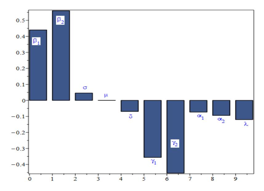
Figure 2 Sensitivity indices for parameters in R0.
The normalized forward sensitivity indices of the basic reproduction number with respect to each of the baseline parameter values is displayed in Figure 2.
3.8 Bifurcation analysis
In this section, we adopt Castillo-Chavez & Song [16] to analyze the bifurcation analysis of Model (2.2). Introducing
\[s = \frac{s(t)}{N} = x_1, e = \frac{E(t)}{N} = x_2, i_1 = \frac{I_1(t)}{N} = x_3, i_2 = \frac{I_2(t)}{N} = x_4,\] \[q = \frac{Q(t)}{N} = x_5, \text{ the system (2) becomes:}\] \[\frac{dx_1}{dt} = \Lambda - \beta_1 x_1 x_3 - \beta_2 x_1 x_4 - \mu x_1 := f_1\] \[\frac{dx_2}{dt} = \beta_1 x_1 x_3 + \beta_2 x_1 x_4 - (\sigma + \mu + \delta) x_2 := f_2\] \[\frac{dx_3}{dt} = \lambda \sigma x_2 - (\gamma_1 + \alpha_1 + \mu + \delta) x_3 := f_3\] \[\frac{dx_4}{dt} = (1 - \lambda) \sigma x_2 - (\gamma_2 + \alpha_2 + \mu + \delta) x_4 := f_4\] (7)
We assume that the bifurcation parameter is . The condition that 0 = 1 implies
\[\lambda = \frac{(\delta^2 + 2\delta\mu + \delta\sigma + \delta\alpha_2 + \delta\gamma_2 + \mu^2 + \sigma\mu + \mu\alpha_2 + \mu\gamma_2 + \sigma\alpha_2 - \sigma\beta_2 + \sigma\gamma_2)(\gamma_1 + \alpha_1 + \mu + \delta)}{\sigma(\delta\beta_1 - \delta\beta_2 + \mu\beta_1 - \mu\beta_2 - \alpha_1\beta_2 + \alpha_2\beta_1 + \gamma_2\beta_1 - \gamma_1\beta_2)} \coloneqq \lambda^*\]
Describing the general system of ODEs such that
\[\frac{dx}{dt} = f(x, \lambda^*), f: \mathbb{R}^n \times \mathbb{R}^n, f \in C^2(\mathbb{R}^n \times \mathbb{R}^n)\]
For the above-described system and for all values of the parameters , it is assumed that zero represents a state of equilibrium, i.e., (0, ∗ ) ≡ 0, ∀ ∗ = 0.
The eigenvalues of the matrix, (0, ∗ ) are given as:
\[s_1 = -\mu, s_2 = -(\theta + \mu + \delta), s_3 = -(\gamma_1 + \alpha_1 + \alpha_2 + 2\mu + 2\delta), s_0 = 0.\]
The right eigenvector of the matrix (0, ∗ ) at zero eigenvalues is:
\[\begin{bmatrix} -\mu & 0 & -\beta_1 & -\beta_2 \\ 0 & -(\sigma + \mu + \delta) & \beta_1 & \beta_2 \\ 0 & \lambda^* \sigma & -(\gamma_1 + \alpha_1 + \mu + \delta) & 0 \\ 0 & \sigma(1 - \lambda^*) & 0 & -(\gamma_2 + \alpha_2 + \mu + \delta) \end{bmatrix} \begin{bmatrix} w_1 \\ w_2 \\ w_3 \\ w_4 \end{bmatrix} = \begin{bmatrix} 0 \\ 0 \\ 0 \\ 0 \end{bmatrix}\]
This implies:
\[\begin{aligned} -\mu w_1 - \beta_1 w_3 - \beta_2 w_4 &= 0 \\ -(\sigma + \mu + \delta) w_2 + \beta_1 w_3 + \beta_2 w_4 &= 0 \\ \sigma \lambda^* w_2 - (\alpha_1 + \gamma_1 + \mu + \delta) w_3 &= 0 \\ \sigma (1 - \lambda^*) w_2 - (\alpha_2 + \gamma_2 + \mu + \delta) w_4 &= 0 \end{aligned}\]
After solving, we have:
\[\begin{split} w_1 &= -\left(\frac{\beta_1 \sigma \lambda^*}{\mu} + \frac{\beta_2 (\alpha_2 + \gamma_2 + \mu + \delta)}{\mu \sigma (1 - \lambda^*) (\alpha_1 + \gamma_1 + \mu + \delta)}\right), \\ w_2 &= \alpha_2 + \gamma_1 + \mu + \delta, w_3 = \sigma \lambda^* \\ w_4 &= \frac{\alpha_2 + \gamma_2 + \mu + \delta}{\sigma (1 - \lambda^*) (\alpha_1 + \gamma_1 + \mu + \delta)}. \end{split}\]
The right eigenvector is:
\[w = \begin{bmatrix} -\left(\frac{\beta_1 \sigma \lambda^*}{\mu} + \frac{\beta_2(\alpha_2 + \gamma_2 + \mu + \delta)}{\mu \sigma (1 - \lambda^*)(\alpha_1 + \gamma_1 + \mu + \delta)}\right) \\ \alpha_2 + \gamma_1 + \mu + \delta \\ \sigma \lambda^* \\ \frac{\alpha_2 + \gamma_2 + \mu + \delta}{\sigma (1 - \lambda^*)(\alpha_1 + \gamma_1 + \mu + \delta)} \end{bmatrix}\]
(8)
Moreover, the left eigenvector \(\mathbf{v} = (v_1, v_2, v_3, v_4)\), accomplishing \(\mathbf{v} * \mathbf{w} = 1\), is given as:
\[-\mu v_1 = 0\] \[-(\sigma + \mu + \delta)v_2 + \sigma \lambda^* v_3 + \sigma (1 - \lambda^*)v_4 = 0\] \[-\beta_1 v_1 + \beta_1 v_2 - (\alpha_1 + \gamma_1 + \mu + \delta)v_3 = 0\] \[-\beta_2 v_1 + \beta_2 v_2 - (\alpha_2 + \gamma_2 + \mu + \delta)v_4 = 0\]
Then the left eigenvector is therefore:
\[v_{1} = 0, v_{2} = \frac{1}{\alpha_{1} + \gamma_{1} + \mu + \delta} - \frac{\alpha_{2} + \gamma_{2} + \mu + \delta}{\alpha_{1} + \gamma_{1} + \mu + \delta} \left[ \beta_{1} \sigma \lambda^{*} - \frac{\beta_{2}}{\sigma (1 - \lambda^{*})} \right],\] \[v_{3} = \beta_{1} (\alpha_{2} + \gamma_{2} + \mu + \delta), v_{4} = \beta_{2} (\alpha_{1} + \gamma_{2} + \mu + \delta)\]
i.e.,
\[v = \left(0.\frac{1}{\alpha_1 + \gamma_1 + \mu + \delta} - \frac{\alpha_2 + \gamma_2 + \mu + \delta}{\alpha_1 + \gamma_1 + \mu + \delta} \left[\beta_1 \sigma \lambda^* - \frac{\beta_2}{\sigma(1 - \lambda^*)}\right], \beta_1(\alpha_2 + \gamma_2 + \mu + \delta), \beta_2(\alpha_1 + \gamma_2 + \mu + \delta)\right)\] \[(9)\]
In a disease-free equilibrium, we estimate the partial derivatives and obtain:
\[\frac{\partial^{2} f_{1}}{\partial x_{1} \partial x_{3}} = \frac{\partial^{2} f_{1}}{\partial x_{3} \partial x_{1}} = -\beta_{1}, \frac{\partial^{2} f_{1}}{\partial x_{1} \partial x_{4}} = \frac{\partial^{2} f_{1}}{\partial x_{4} \partial x_{1}} = -\beta_{2},\] \[\frac{\partial^{2} f_{2}}{\partial x_{1} \partial x_{3}} = \frac{\partial^{2} f_{2}}{\partial x_{3} \partial x_{1}} = \beta_{1}, \frac{\partial^{2} f_{2}}{\partial x_{1} \partial x_{4}} = \frac{\partial^{2} f_{2}}{\partial x_{4} \partial x_{1}} = \beta_{2},\] \[\frac{\partial^{2} f_{3}}{\partial x_{2} \partial \lambda} = \sigma, \quad \frac{\partial^{2} f_{4}}{\partial x_{2} \partial \lambda} = -\sigma,\] while the remaining second-order derivatives go to zero.
Coefficients \(\boldsymbol{a}\) and \(\boldsymbol{b}\) are calculated using the definition given by Castillo-Chavez and Song [16], i.e., assuming that \(f_k\) is the k-th component of f and
\[\mathbf{a} = \sum_{k,i,j=1}^{4} v_k w_i w_j \frac{\partial^2 f_k}{\partial x_i \partial x_j} (\xi_0, \lambda^*)\]\[\mathbf{b} = \sum_{k,i,j=1}^{4} v_k w_i \frac{\partial^2 f_k}{\partial x_i \partial \lambda} (\xi_0, \lambda^*)\]
The local dynamics of Model 2 are entirely estimated by the coefficients \(\bf a\) and \(\bf b\) around x=0. Taking into consideration the system of equations (7) and estimating the coefficients a and b, all derivative terms other than zero for \(\frac{\partial^2 f_k}{\partial x_i \partial x_j}(\xi_0, \lambda^*)\) and \(\frac{\partial^2 f_k}{\partial x_i \partial \lambda}(\xi_0, \lambda^*)\) are as follows:
\[\boldsymbol{a} = 2v_1 w_1 w_3 \frac{\partial^2 f_1}{\partial x_1 \partial x_3} (\xi_0, \lambda^*) + 2v_1 w_1 w_4 \frac{\partial^2 f_1}{\partial x_1 \partial x_4} (\xi_0, \lambda^*) + 2v_2 w_1 w_3 \frac{\partial^2 f_2}{\partial x_1 \partial x_3} (\xi_0, \lambda^*) + + 2v_2 w_1 w_4 \frac{\partial^2 f_2}{\partial x_1 \partial x_4} (\xi_0, \lambda^*)\] and
\[b = v_4 w_2 \frac{\partial^2 f_4}{\partial x_1 \partial \lambda} (\xi_0, \lambda^*)\]
Using Equations (8) and (9) with some partial second-order derivatives obtained from System (7), we get:
\[a = \frac{2(\lambda^* \sigma^2 \beta_1 (\lambda^* - 1) + \beta_2) MN}{3\sigma\mu(\lambda^* - 1)^3 (\gamma_1 + \alpha_1 + \mu + \delta)^2} > 0\] where
\[M = ((\lambda^* - 1)\{\lambda^* \sigma^2 \beta_1 (\gamma_2 + \alpha_2 + \mu + \delta) + \sigma\} + \beta_2 (\gamma_2 + \alpha_2 + \mu + \delta))\] and
\[N = ((\lambda^* - 1)\lambda^*\sigma^2\beta_1(\gamma_1 + \alpha_1 + \mu + \delta) - (\gamma_2 + \alpha_2 + \mu + \delta))\]
Also,
\[\mathbf{b} = -\sigma \beta_2 (\gamma_1 + \alpha_1 + \mu + \delta)^2 < 0.\]
It can be seen that a is a positive coefficient, while b is a negative coefficient. According to Castillo-Chevez & Song [16], if a > 0, b < 0 when \(\lambda^* < 0\), the system is unable to maintain its stability and there exists a negative and locally asymptotically stable negative equilibrium.
Define:
\[R_0^{**} = \frac{\beta_1 \lambda^* \sigma}{(\sigma + \mu + \delta)(\gamma_1 + \alpha_1 + \mu + \delta)} + \frac{\beta_1 (1 - \lambda^*) \sigma}{(\sigma + \mu + \delta)(\gamma_2 + \alpha_2 + \mu + \delta)}.\]
If \(R_0^{**} < 1\), then a < 0 and if \(R_0^{**} > 1\), then a > 0. Therefore, the following follows: if \(R_0^{**} > 1\), the first four equations in System (2) exhibit backward bifurcation when \(R_0 = 1\). If \(R_0^{**} < 1\), the first four equations in System (2) exhibit forward bifurcation when \(R_0 = 1\).
4 Numerical Simulation
We devote this section to performing a numerical simulation of the formulated two-strain Covid-19 model. The model is solved numerically in R using the deSolve package. The estimated and fitted parameters utilized in the simulation process are given in Table 1. Susceptible, Exposed, Infected by Strain 1, Infected by Strain 2, Quarantine and Recovery at initial time t=0 are given respectively as: \(S(0)=3978, E(0)=7000, I_1(0)=4000, I_2(0)=2500, Q(0)=4000\) and R(0)=0. We assume there are no recovered individuals at the initial level.
| Parameter | Description | Value | Source |
|---|---|---|---|
| μ | Natural death rate | 0.000422536 | Estimated |
| λ | Fraction of individuals infected by Strain 1 | 0.5 | Estimated |
| \(\beta_1\) | Transmission rate to Strain 1 | \(\frac{1}{14}\) | Estimated |
| \(\beta_2\) | Transmission rate to Strain 2 | \(\frac{1}{11}\) | Estimated |
| δ | Death rate due to Strain 1 or 2 | 0.0276 | Estimated |
| σ | Progression rate to the Infectious compartment from the Exposed compartment | \(\frac{1}{7}\) | Estimated |
| \(\gamma_1, \gamma_2\) | Recovery rates from the Infectious compartment | 0.97 | Estimated |
| \(\alpha_1, \alpha_1,\) | Detention rates from the Infectious compartment to the Quarantine compartment | 0.2 | [17] |
| \(\theta\) | Recovery rate from the Quarantine compartment | \(\frac{1}{12}\) | Estimated |
Table 2 Parameter values for the Covid-19 model.
The results obtained from the numerical simulation are depicted in the figures below. Figure 3 presents an overview of what happens in the five compartments. The figure shows that more people recovered from the two strains and the epidemic curve flattened after some time. The number of quarantine compartments increased from the starting day and reached its peak at the end of the fifth day. After the fifth day, the number of individuals in the Quarantine compartment decreased. It can also be seen that the Strain 1 and Strain 2 compartments decreased until day 20, when the number of people in that compartment was reduced to zero. The number of people who were exposed to the disease also declined, as can be seen in the figure, whereby we experience more recovery. The number of susceptible individuals slightly decreased at the start and remained steady throughout.
Figure 4 shows that the number of individuals in the Infected compartments of Strain 1 and Strain 2 rose for a period before they started declining, while the Exposed compartment decreased.
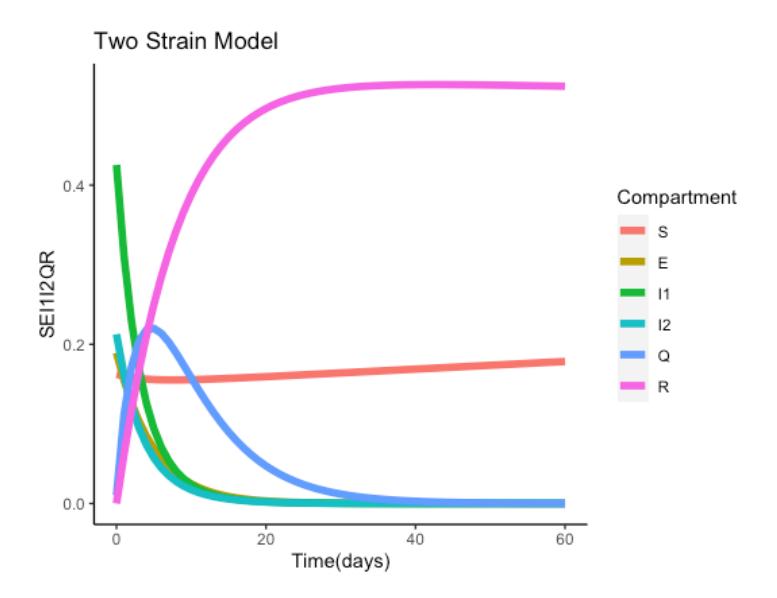
Figure 3 Dynamic of the six compartments.
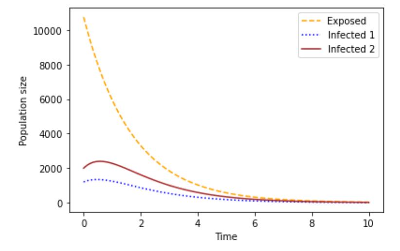
Figure 4 Behavior of Exposed, Strain 1 and Strain 2.
Figures 5-7 shows the impacts of increasing , 1 and 2 on recovery. It can be seen in Figure 5 that as the progression rate increased there existed an increase in the Recovery compartment at all times. This implies that more people recovered when they contracted the disease. The impact of the transmission rate of Strain 2 is investigated in Figure 6. We notice that at first there is no difference, but as time goes on, an increase in the transmission rate of Strain 2 appears. We notice that more people recovered. The same also applied to Strain 1, as shown in Figure 7.
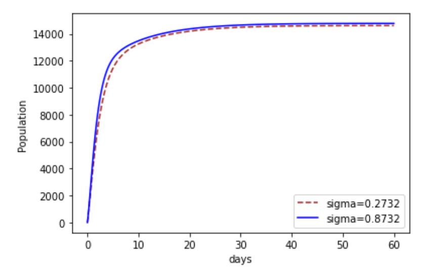
Figure 5 The effect of increasing on recovery.
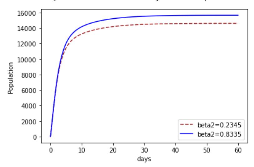
Figure 6 The effect of increasing 2 on recovery.
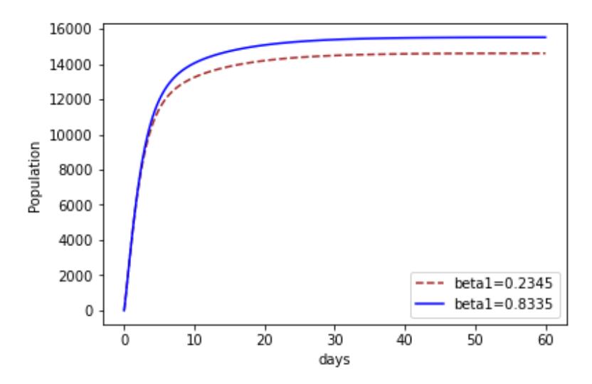
Figure 7 The effect of increasing \(\beta_1\) on recovery.
5 Conclusions
We considered a system of mathematical equations that reports the dynamics of two COVID-19 strains without control or treatment. The analysis of the system was well established. We presented a stability analysis of the disease-free equilibrium and the endemic equilibrium based on the estimated basic reproduction number. Whenever \(R_0 < 1\), the disease-free equilibrium is locally asymptotically stable and it is globally asymptotic stable if and only if \(L'(S, E, I_1, I_1) < 0\). We presented a bifurcation analysis for the formulated problem and concluded that if \(R_0^{**} > 1\), the first four equations in System (2) exhibit backward bifurcation when \(R_0 = 1\). If \(R_0^{**} < 1\), the first four equations in System (2) exhibit forward bifurcation when \(R_0 = 1\). We also presented a numerical simulation to see the dynamics of the six compartments and the impact of some parameters on recovery.