
1 Introduction
An S-wave velocity profile is an essential mechanical parameter in geophysics because it corresponds to the material's shear strength and can delineate lithological variation in the subsurface [1-3]. It is widely used to study materials in deep structures, from the crust and upper mantle [4,5] to the uppermost crust
Received September 21st, 2022, Revised May 11th, 2023, Accepted for publication May 24th, 2023 Copyright © 2022 Published by ITB Institut for Research and Community Service, ISSN: 2337-5760, DOI: 10.5614/j.math.fund.sci.2023.54.3.4
[6,7]. Shallow S-wave velocity profiles are particularly preferred in the earthquake engineering field to evaluate the presence of soft soil layers above a hard bedrock layer, which are responsible for soil amplification of earthquake ground motion on the surface. The seismic site characterization of an area can be investigated from soil amplification features [8-10].
Shallow S-wave-velocity profiles can be directly estimated using P-S logging in a borehole or in active seismic experiments. However, these methods are expensive when obtaining profiles from numerous boreholes or doing elaborate surveys in large areas. Recently, surface wave methods [11,12], including methods using microtremor exploration, have come into widespread use for estimating S-wave velocity profiles at relatively low costs, with faster data processing, and more environmental-friendly methods than borehole logging.
Among the available surface wave methods, the microtremor horizontal-tovertical spectral ratio (HVSR) technique has gained popularity due to its ease of use in field measurements. The spectral ratio can be calculated from horizontal and vertical components of microtremor records at a single station for site amplification [13]. The possibility of utilizing the microtremor HVSR to estimate S-wave velocity profiles was first investigated by Nogoshi and Igarashi [14] based on the similarity between the HVSR and the ellipticity of the fundamental mode Rayleigh wave. Since then, this possibility has been confirmed by other studies [15,16], and the technique has since been widely used to retrieve 1D S-wave velocity profiles [17-20]. In the HVSR analysis, the 1D profile is represented as a horizontally-layered model. The S-wave velocity and the thickness of each layer are determined using inversion. However, it is sometimes difficult to choose the appropriate number of layers and the initial model. This may be solved by applying a simplified profile representation with reduction of the number of model parameters. Several studies have used velocity-depth functions of S-wave velocity in a surface layer over a half-space for the HVSR analysis [21,22]. The only model parameters needed for the profile are the surface S-wave velocity and the velocity gradient of the velocitydepth function. Therefore, S-wave velocity profile estimation using the HVSR can be done by minimizing the misfit between the observed HVSR and the theoretical one using a grid search. However, the usage of the observed HVSR amplitude is not straightforward, since the amplitude is controlled by a contribution of the Rayleigh and Love waves, which may vary at each site [23]. Velocity-depth functions have also been used to establish the empirical relations between sediment thicknesses and observed HVSR peak frequencies. Ibs-von Seht and Wohlenberg [24] conducted a mapping of the sediment thickness from observed HVSR spectra in the western Lower Rhine Embayment in Germany. The study used a fixed surface velocity and a fixed velocity gradient of the velocity-depth function from a priori information. This method was also applied by Parolai et al. in [25] and D'Amico et al. in [26] to assess the thickness of sediments. Recently, Thabet [27,28] constructed regional relationships between peak frequencies and sediment thicknesses using more than 10,000 weak earthquake HVSRs recorded nationwide by seismographs in Japan. However, this method cannot accommodate local velocity variation as it causes errors in anticipating the soil amplification. Several velocity-depth functions are available in the profile representations. For example, linear S-wave velocity increments were observed in the Holocene Bay mud sediment in Oakland, California [29] and in soil deposits at the Shimousa deep borehole observatory, Japan [30]. The power-law of S-wave velocity increment was observed at both Tertiary sediment in the Cologne area in Germany [25] and Quaternary-Tertiary sediment in the Almaty Basin, Kazakhstan [31]. However, based on KiK-net site profiles in Japan, Wang et al. [32] concluded that a profile represented by a linear S-wave velocity increment performs better than a profile expressed with a power-law velocity increment to predict fundamental peak frequencies.
In this study, we propose a simplified method for deducing S-wave velocity (Vs) profiles with the assumption of a surface layer that has a constant velocity gradient. We used the measured surface S-wave velocity to accommodate local velocity variation at each site. Consequently, the velocity gradient is uniquely estimated from the peak frequency of the observed microtremor HVSR. We used the peak frequency instead of its amplitude for a robust estimation of the gradient. We assessed the applicability of the proposed method in numerical tests. We then applied the method to actual data from the Bandung Basin, Indonesia to determine shallow soil profiles. Furthermore, the estimated profiles were compared with the results from conventional microtremor array surveys.
2 Method
We assume that the velocities of the Vs profile increase linearly from the surface to the depth of the top of the bedrock, as illustrated in Figure 1c and expressed in Eq. (1) [32-34]:
\[Vs(z) = V1 + bz\], for \(0 \le z < z_B\)
= \(V_B\), for \(z \ge z_B\) (1)
where
\[z_{\rm B} = \frac{V_B - V_1}{b}\] where V1, b, z and VB are surface S-wave velocity, velocity gradient, depth of profile, and bedrock S-wave velocity, respectively. ZB is the depth to the bedrock, which is derived from a linear function. Here, we define the bedrock as engineering bedrock, a hard layer beneath soil layers in the near-surface with Swave velocity larger than 400 m/s [35]. Essentially, the profile parameters are the surface S-wave velocity, the velocity gradient, and the S-wave velocity of the bedrock. Here, we give the bedrock S-wave velocity by considering a priori information from geological or geophysical surveys. Thus, the profile can be estimated using V1 and the velocity gradient.
The concept of the proposed model parameterization to estimate 1D S-wave velocity profiles is illustrated in Figure 1. We assume that V1 is the same as the observed value of the fundamental mode Rayleigh wave phase velocity at a sufficiently high frequency of its dispersion curve. Accordingly, V1 can be measured from active seismic measurement. In our experiment, a number of geophones were set in a short surveying line to observe only the phase velocity of the Rayleigh wave at high frequencies from an impact source. The measurement with a few geophones is simpler than conventional seismic or surface-wave methods for phase velocity in a wide frequency range. Up to six to eight geophones can be set up in a short surveying line with a spacing of 1 m. The number of deployed geophones is one-third to a quarter of the common number of geophones used in conventional methods. Considering the guideline of an active seismic survey [36], we anticipated that wavelengths of 2 to 7 m for high-frequency phase velocities could be observed from this arrangement. Since we intended to observe the phase velocity at a high frequency in our measurements, the observed phase velocity was insufficient in frequency range for a conventional phase velocity inversion. We also took into consideration that the observed Rayleigh wave phase velocity at high frequency may be contaminated by higher modes with larger values than those of the fundamental mode [36,37]. Therefore, we could also use the minimum value of the observed phase velocities as the V1 for the fundamental mode of the Rayleigh wave.
Next, we determined the velocity gradient using the peak frequency of the observed microtremor HVSR. The observed microtremor HVSR peak frequency was used to tune and validate the thicknesses of the Vs profile, because the peak frequency of the microtremor HVSR is consistent with the peak frequency of the theoretical ellipticity of the fundamental mode Rayleigh wave [15,38]. Since observing the HVSR peak frequency is crucial in the proposed method, we considered that the peak HVSR should have an amplitude higher than two [39]. We determined the gradient from the agreement of the peak frequencies between the observed HVSR and the theoretical ellipticity of the fundamental mode of the Rayleigh wave in a linear model with the measured V1 and the given bedrock velocity. In the theoretical ellipticity
calculation, we discretized the linear model into numerous thin layers, each with a thickness of 0.1 m. We used a one-dimensional grid search procedure of minimum misfit for the peak frequencies. It should be noted that the theoretical ellipticity of the estimated Vs profile has only one single peak frequency as a consequence of using a linear profile representation. However, we may observe the HVSR having several peak frequencies [28,40]. In such cases, we chose the observed HVSR peak at the highest frequency, representing a shallow Vs profile, for the velocity gradient estimation. Hereafter, we refer to the proposed method as V1-HVSR.
The V1-HVSR method offers a simpler procedure than the conventional microtremor array survey for shallow Vs profile estimation. The instrument used for the V1-HVSR method is a conventional and inexpensive geophone with a natural frequency of 4.5 Hz. The method only requires a small number of geophones and a three-component microtremor sensor, whereas a conventional microtremor array survey requires expensive broad-band instruments. Furthermore, the array survey requires several measurements with differentsized arrays to obtain observed phase velocities in a wide frequency range. Therefore, the V1-HVSR method requires less effort in making the measurements and less data processing than conventional methods.
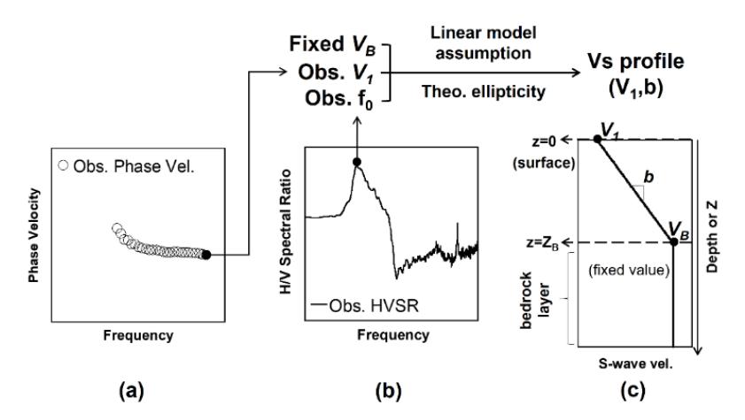
Figure 1 Illustration of the proposed method using the surface S-wave velocity (V1) and the peak frequency (f0) of the microtremor HVSR. a) V1 is estimated based on the minimum value of the Rayleigh wave phase velocity at a high frequency range, using a short-length active seismic measurement. b) The velocity-depth gradient (b) in the profile, which is represented by a linear model with a given bedrock velocity (VB), is determined by the fit of the peak frequencies between the theoretical ellipticity of the fundamental mode of the Rayleigh wave and the observed HVSR. c) Representation of an estimated Vs profile from this method. ZB corresponds to the depth of the bedrock layer.
3 Numerical Tests
3.1 Borehole Profiles in Bandung Basin
We conducted numerical tests to examine the applicability of the proposed method. Since we later applied the method to actual data from the Bandung Basin, we referred to samples of the borehole profiles in the basin in the numerical tests. The surface geology of the Bandung Basin is shown in Figure 2. The basin is mostly filled with thick Quaternary lacustrine sediments and the intercalation of volcaniclastic sediments [41,42]. Since shallow S-wave velocity profiles from downhole or P-S logging measurements were unavailable for the basin, we utilized three borehole profiles that only contained soil type information from the geomorphological and sedimentological studies of the basin [41,43]. The locations and descriptions of the boreholes are shown in Figures 2 and 3, respectively. The boreholes were located in parts covered by the Quaternary layers.
The Quaternary lacustrine sedimentation begins at depths of 46 m, 48 m, and 50 m in boreholes 1, 2, and 3 [41,43], as shown in Figure 3. Eruptions of a northern volcano produced volcaniclastic sediments that intercalate the lacustrine sediments. The sedimentation of the volcaniclastic deposits reaches depths of 12 m, 31 m, and 38 m in boreholes 1, 2, and 3, respectively. The soil deposits are dominated by lacustrine sedimentation above volcaniclastic sediments.
The soil data of the boreholes were further used to assume Vs profiles for the numerical tests. We employed an existing empirical equation proposed by Ohta and Goto in [44] to convert the soil type information to S-wave velocity. This empirical relation was used in [45] to convert the soil profile in Jakarta to Swave velocities. However, the choice of the empirical equation to generate the velocity profile is not crucial in this study, because we only used assumed Vs profiles in the numerical tests to confirm the applicability of the proposed method. Here, we utilized Eq. (2) proposed by Ohta and Goto in [44]. The Swave velocity at a depth of z, Vs(z), is calculated from:
\[Vs(z) = 78.98 z^{0.312} SF\] (2)
where SF is the soil type factor. The values of SF are listed in Table 1. Since the empirical equation gives a null velocity at a depth of 0 m, we set 1 m for z in Eq. (2) to calculate S-wave velocity at depths from 0 to 1 m. We also used a soil factor of 1.0 at these depths, as they are clay layers. The S-wave velocity at these depths was 79 m/s for all the boreholes.
We can identify two main boundaries in the soil profiles, as illustrated by representative soil columns in Figure 3. The first boundary is set between the lacustrine sediments and the volcaniclastic sediments at depths of 12 m, 31 m, and 38 m in boreholes 1, 2, and 3, respectively. The S-wave velocities of the lacustrine sediments with thick organic silt and clay layers start from 79 m/s to 171 m/s, 230 m/s, and 246 m/s in boreholes 1, 2, and 3. We set a soil type factor of 1.352 as the average of the factors of soil types medium sand and coarse sand for the volcaniclastic sediment layers. We could identify the top of the gravelly sand layers at depths of 46 m, 48 m, and 50 m in boreholes 1, 2, and 3, respectively. The gravelly sand layers are regarded as bedrock layers with Swave velocities of 508 m/s, 515 m/s, and 521 m/s in boreholes 1, 2, and 3, respectively. This was calculated from the empirical equation using the top depths and a soil type factor of 1.948 as the average of the factors of soil types sand and gravel, and gravel. The corresponding S-wave velocities of the assumed borehole profiles are summarized in Table 2 and depicted as solid lines in Figure 4.
Table 1 Soil type factors in Eq. (2) [44].
| Soil type | SF |
|---|---|
| Clay | 1.000 |
| Fine sand | 1.260 |
| Medium sand | 1.282 |
| Coarse sand | 1.422 |
| Sand and gravel | 1.641 |
| Gravel | 2.255 |
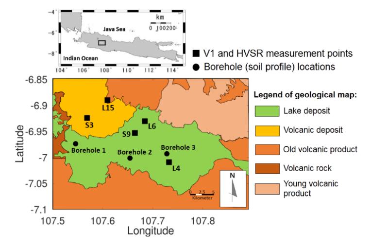
Figure 2 Surface geological map of the Bandung Basin, simplified from Dam and Suparan [43]. The black circles and square marks indicate the location of the
boreholes and V1-HVSR measurement sites, respectively. The location of the Bandung Basin is shown as a rectangle in the upper map.
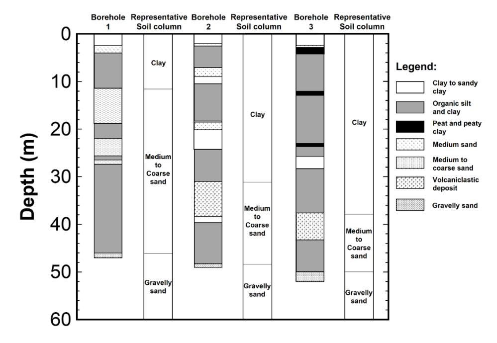
Figure 3 Soil columns of the boreholes in the Bandung Basin. Borehole 1 was taken from Dam and Suparan [43], while boreholes 2 and 3 were taken from Dam et al. [41]. The borehole profiles are primarily composed of three soil types: clay, medium to coarse sand, and gravelly sand. The borehole locations are shown in Figure 2.
Table 2 Assumed S-wave velocity profiles of the soil columns in the Bandung Basin used for the numerical tests.
| Layer | S-wave velocity (m/s) | Layer thickness (m) | Density | Soil type | ||||
|---|---|---|---|---|---|---|---|---|
| Br. 1 | Br. 2 | Br. 3 | Br. 1 | Br. 2 | Br. 3 | (g/cm3) | 3 T 3 P 3 | |
| First | 78.98 z0.312 | 12 | 30.8 | 38 | 1.5 | Clay | ||
| Second | 106.78 z0.312 | 34 | 17.2 | 12 | 1.7 | Medium to coarse sand | ||
| Bedrock | 508 | 515 | 521 | - | - | - | 1.8 | Gravelly sand |
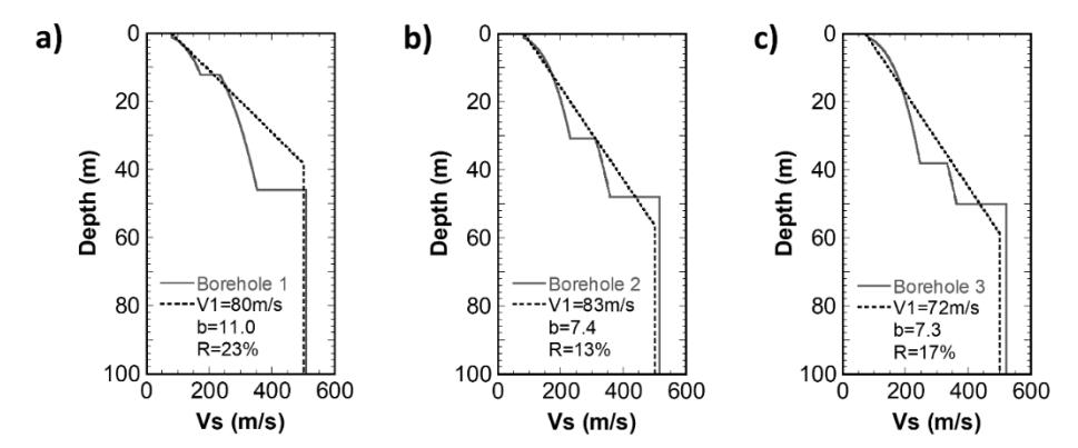
Figure 4 Vs profile comparison at: a) borehole 1, b) borehole 2, and c) borehole 3. Solid gray and black dashed lines indicate the velocities of the assumed borehole profiles estimated by the empirical relation between soil type and Swave velocities and estimated Vs profiles using the proposed method. The Rvalue of each Vs profile is indicated in each plot.
3.2 Generation of Synthetic Data
We calculated synthetic ellipticities of the fundamental mode Rayleigh wave for three assumed Vs profiles, as shown in Figure 5. The ellipticities were calculated with the method proposed by Haskell in [46]. P-wave velocities (Vp) were derived from S-wave velocities (Vs) using the empirical relationship proposed by Kitsunezaki et al. in [47]:
\[Vp = 1.11Vs + 1290 (3)\] with Vp and Vs in m/s. Eq. (3) has also been used for Vs profiling using the HVSR in previous studies [19,48]. We then contaminated the peak frequency of the calculated ellipticities with ±10% random noise to generate synthetic observed peak frequencies. The synthetic observed peak frequencies of the ellipticities were 2.5, 1.7, and 1.5 Hz in boreholes 1, 2, and 3, respectively.
Since V1 is retrieved from the phase velocity of the fundamental mode of the Rayleigh wave at a high frequency, we also calculated synthetic phase velocities of the fundamental mode of the Rayleigh wave in the assumed Vs profiles, as shown in Figure 6. The phase velocity for all the profiles is convergent to a velocity of 78 m/s at a frequency of 40 Hz. We then set the synthetic observed V1s as 80, 83, and 72 m/s for boreholes 1, 2, and 3 after addition of ±10% random noise to the convergent phase velocity at a frequency of 40 Hz. The contamination of ±10% random noise for the phase velocity was referenced from a previous numerical test [49].
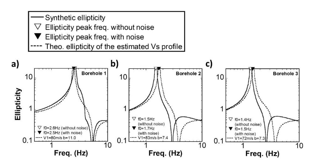
Figure 5 Theoretical ellipticities of Rayleigh wave surface motion at: a) borehole 1, b) borehole 2, and c) borehole 3 cases. Solid and dashed lines correspond to the synthetic fundamental mode of the Rayleigh wave ellipticity from the Vs profiles of the boreholes, as shown in Table 2, and the ellipticity of the estimated Vs profiles, respectively. White and black inverted triangles indicate the peak frequencies of the synthetic ellipticities of the borehole profiles, and the synthetic observed ellipticity peak frequency used for profile estimation, respectively.
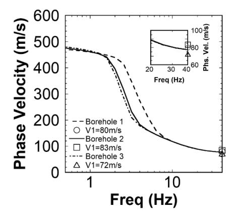
Figure 6 Theoretical phase velocities of borehole Vs profiles with synthetic observed V1s. Dashed, solid, and dash-dotted lines correspond to the synthetic phase velocities of the fundamental mode of Rayleigh waves from Vs profiles of boreholes 1, 2, and 3 in Table 2, respectively. The circle, square, and triangle markings correspond to the synthetic observed V1s used in the numerical tests at boreholes 1, 2, and 3, respectively. The synthetic observed V1 was generated from the contamination of ±10% random noise in the synthetic phase velocity at 40 Hz. The small panel shows the high-frequency range of the phase velocity.
3.3 Profile Estimation
We applied the proposed method to the above-mentioned synthetic observed data. We set the bedrock velocity at 500 m/s as common S-wave velocity for the engineering bedrock, which was assumed for shallow S-wave velocity profiling in previous microtremor array surveys [50,51]. The effects of various S-wave velocities of the bedrock in the profile estimation will be examined later. The gradient at each borehole was estimated using the synthetic observed peak frequency. The dashed lines in Figure 5 show the estimated gradients based on fitting the synthetic observed peak frequencies to calculated ones. The estimated gradients were 11.0, 7.4, and 7.3 m/s/m for boreholes 1, 2, and 3, respectively.
The estimated Vs profiles for each site are shown by a dashed line in Figure 4 in comparison to the assumed Vs borehole profile. We observed that the velocity variation in the first layer of the assumed profile of borehole 1 was well-approximated with the estimated Vs profile. Meanwhile, the velocities at depths of 20 to 46 m in the estimated Vs profile were higher than those in the assumed Vs profile for borehole 1. The estimated Vs profiles at boreholes 2 and 3 corresponded well with the velocity distributions of the first and second layers of the assumed Vs borehole profiles. However, the deep parts of the estimated Vs profiles had lower velocities than those of the assumed Vs profiles at a depth of 48 m for borehole 2, and at a depth of 50 m for borehole 3. We also observed that the bedrock depths were inaccurate in the estimated Vs profiles of all boreholes. The estimated Vs profile at borehole 1 had a shallower bedrock depth, while the bedrock depths at boreholes 2 and 3 were deeper than those of the assumed Vs profiles.
Furthermore, we calculated the average relative difference (R), as defined by Xia et al. in [52] to quantify the differences between the assumed and the estimated Vs profiles from:
\[R = \frac{100}{n} \sum_{k=1}^{n} \left( \frac{\left| V_{br_k} - V_{c_k} \right|}{V_{br_k}} \right)\] (4)
where \(V_{br_k}\) is the S-wave velocity of the borehole profile at the k-th depth, \(V_{c_k}\) is the S-wave velocity of the estimated Vs profile at the same depth, and n is the number of depth samplings of the profile every 1 m. We included all the S-wave velocities of the borehole profiles above the bedrock depth \((0 \le z < z_B)\) for calculating the Rs. Therefore, the maximum n in Eq. (4) will be controlled by the bedrock depth of the borehole profile.
Comparisons between the estimated and the assumed borehole profiles can be categorized into three groups with the R values, as described by Xia et al. in [52]. An R value equal to or less than 10% indicates an excellent agreement between two profiles. The second category is good agreement, which is defined as an R value between 10% and 20%. Fair agreement is determined if an R value is greater than 20%. The R values of the three cases were 23%, 13%, and 17% for boreholes 1, 2, and 3, respectively. The estimated Vs profile at borehole 1 can be categorized as fair agreement, while the estimated Vs profiles at boreholes 2 and 3 can be classified as good agreement. Thus, we can confirm that the proposed method can be applied to retrieve 1D Vs profiles with good agreement.
4 Application to Actual Data in Bandung Basin
We applied the proposed method to actual data obtained at five sites in the Bandung Basin. The sites were located in the deposit areas in the basin. L15 and S3 were located on the volcanic deposits in the northwestern part, while L4, L6, and S9 belonged to the area covered with lacustrine deposits in the central part, as shown in the surface geological map in Figure 2. The locations and names of the sites are referred to in previous microtremor array surveys in the Bandung Basin [53]. In this study, we conducted field measurements to obtain V1 and the microtremor HVSR at each site.
4.1 Measurement of V1 and Microtremor HVSR
We conducted short-length active seismic measurements to obtain the V1s. We arranged seven vertical geophones with a natural frequency of 4.5 Hz in a surveying line with an interval of 1 m. Therefore, the line array was expected to record waves with wavelengths of 2 to 6 m for obtaining high-frequency phase velocities based on active seismic measurement guidelines (e.g., [36]). An impact source by sledgehammer was placed at an offset distance of 5 m from the end of the line array. We recorded the waveforms with a sampling frequency of 2 kHz. The observed waveforms were transformed into a frequency-phase velocity (f-c) spectrum using the frequency-wavenumber (f-k) transformation [54] to retrieve the Rayleigh wave phase velocity. The phase velocity was calculated by dividing the angular frequency by the wavenumber. We could then identify the dispersion curve of the observed Rayleigh wave phase velocity from the high amplitude part of the f-c spectrum. Finally, the V1 was decided as the observed Rayleigh wave phase velocity at a high frequency. Alternatively, we picked up the minimum phase velocity if the observed dispersion curve showed inverse dispersive features.
We also measured the microtremors by installing a three-component sensor near the surveying line. According to the SESAME HVSR analysis guideline [55], 10 windows of 40 seconds are required to obtain a reliable HVSR peak frequency larger than 0.5 Hz. Hence, we recorded microtremors for 10 to 15 minutes with a sampling rate of 100 Hz. We selected several stationary segments without transient noise with a length of 40.96 or 81.92 seconds to compute the HVSR. We calculated the Fourier spectra of the three components at each segment using a Parzen window with a bandwidth of 0.1 Hz for smoothing. The HVSR was obtained as the ratio of the quadratic mean of the two horizontal spectra to the vertical spectrum. Lastly, we averaged the HVSRs of all the segments to obtain the final HVSR.
4.2 Results of Measurements
The results of the active seismic surveys for L4, L6, L15, S3, and S9 are shown in Figures 7 and 8. An example of the recorded waveforms at L4 and its corresponding f-c spectrum are shown in Figures 7a and 7b. We could observe the fundamental mode of the Rayleigh wave, which is characterized by a high amplitude of the spectrum at a frequency range of 15 to 45 Hz in Figure 7b. Meanwhile, the higher mode of Rayleigh wave phase velocity was also identified at frequencies higher than 45 Hz. To identify the V1, we picked up the fundamental mode of the observed Rayleigh wave phase velocity from the maximum amplitude of the spectrum for each frequency, as indicated by circles and black dashed lines in Figure 7b. We estimated the V1 for the fundamental mode of the Rayleigh wave phase velocity at a high-frequency of 50 Hz at L4 as 70 m/s. As shown in Figure 8, we observed an inverse dispersive trend of the observed phase velocity at frequencies higher than 25 Hz at L6 and higher than 30 Hz at S3, indicating the dominant higher modes. The V1s were selected from the minimum phase velocities to consider only the contribution of the fundamental mode at the sites. The estimated V1s from the minimum phase velocities at L6 and S3 are 105 m/s at a frequency of 20 Hz and 140 m/s at a frequency of 25 Hz, respectively. Moreover, the f-c spectra at L15 and S9 showed normal dispersive features of the observed phase velocities. The phase velocity of the fundamental mode of the Rayleigh wave at L15 ranged between 240 m/s at a frequency of 12 Hz and 150 m/s at a frequency of 62 Hz. Meanwhile, the phase velocity at S9 ranged between 190 m/s at a frequency of 14 Hz and 120 m/s at a frequency of 82 Hz. We estimated a V1s of 150 m/s at L15 and 120 m/s at S9, respectively.
The observed HVSRs at the five sites with their standard deviations are shown in Figure 9. The peak frequencies of the HVSRs were 0.6 Hz at L4 and 0.9 Hz at L6, respectively. The HVSRs at L15, S3, and S9 had peak frequencies of 7, 7, and 8 Hz, respectively. These peak frequencies are indicated by triangles in Figure 9.
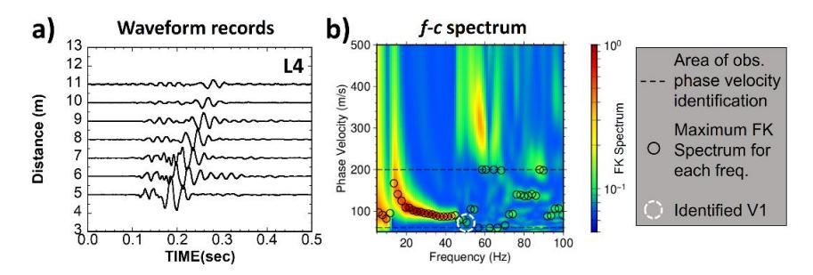
Figure 7 Example of V1 estimation at L4. a) Observed waveforms from active seismic measurement, b) f-c spectrum of the observed waveforms and the observed Rayleigh wave phase velocity. Black dashed lines represent the f-c spectrum area picked to observe the Rayleigh wave phase velocity. Black circles correspond to the maximum amplitude of f-k spectrum for each frequency to identify the phase velocity. The large white dashed circle indicates the observed V1. The amplitude of the f-k spectra is illustrated in color scale.
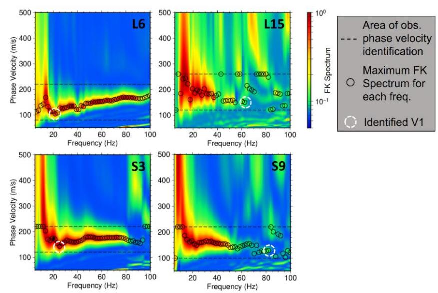
Figure 8 Observed frequency-phase velocity (f-c) spectra with Rayleigh wave phase velocities from active seismic measurements at L6, L15, S3, and S9. Black dashed lines represent the f-c spectrum area picked to observe the phase velocity. Black circles correspond to the maximum amplitude of the f-k spectrum for each frequency to identify the observed Rayleigh wave phase velocity. The large white dashed circles indicate the observed V1. The amplitude of the f-k spectra is illustrated in the color scale.
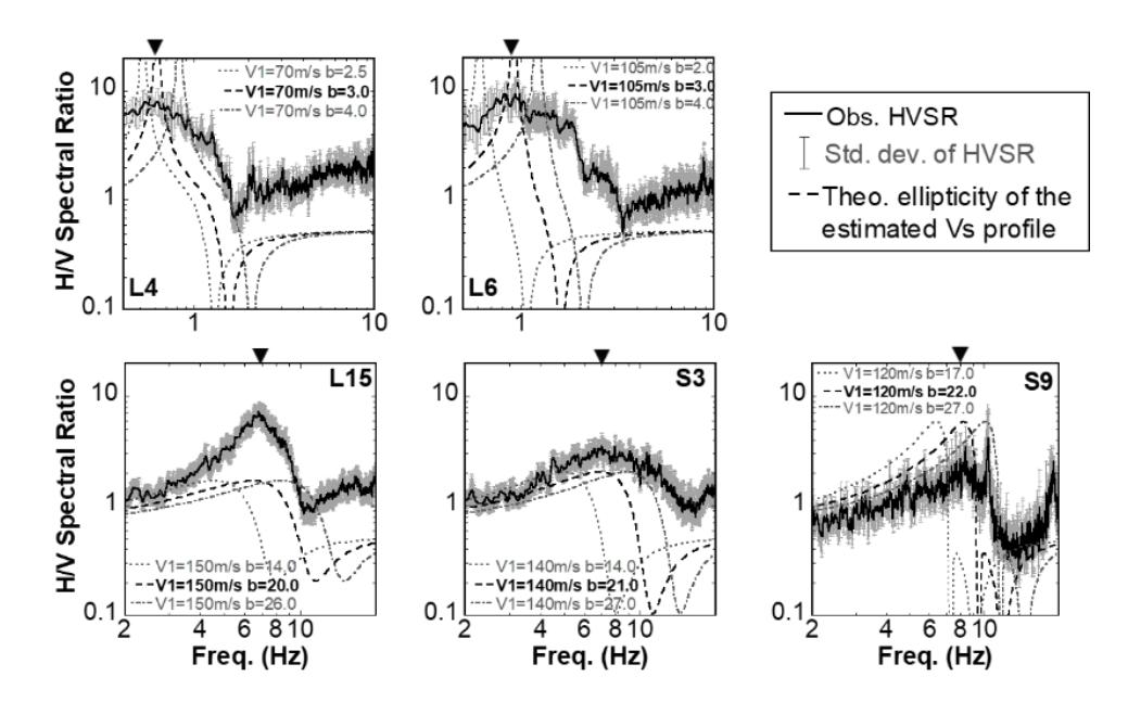
Figure 9 The HVSR spectra for determining gradient (b) at each measurement site. Solid black and gray thin lines indicate observed HVSRs with their standard deviations. The gray dashed, gray dash-dotted, and black dashed lines represent theoretical ellipticity of the fundamental mode Rayleigh wave, using measured V1 with low b, high b, and optimal b, respectively. The black inverted triangles indicate the peak frequency of the observed HVSR.
4.3 Determination of Vs Profiles
The measured V1s and the peak frequencies of the HVSRs were used to determine gradients, as shown in Figure 9. The gradients were determined from a grid search for a peak frequency of theoretical ellipticity that is similar to the observed HVSR peak frequency. The measured V1 and a given bedrock velocity of 500 m/s with velocity gradients were used to calculate the theoretical ellipticities. We searched for the optimal velocity gradient from the grid search. Since the gradient controls the thickness of the profile, a smaller gradient corresponds to a larger profile thickness (see ZB in Eq. (1)). Therefore, the ellipticity for a profile with a small gradient shows a peak at a low frequency in Figure 9. Moreover, the amplitude of theoretical ellipticities at each site does not change after adjusting the gradient (b), because each theoretical ellipticity has a similar velocity contrast between the surface and bedrock velocities.
The Vs profiles estimated at all the sites are displayed in Figure 10. We found that the estimated Vs profiles at L15, S3, and S9 had similar features, characterized by thin sediment layers. The gradients estimated at these sites were 20, 21, and 22 m/s/m, respectively. On the other hand, the Vs profiles at L4 and L6, were characterized by thick sediment layers, with small gradients of 3 m/s/m. The Vs profile at L4 had a lower S-wave velocity than the profile at L6 due to a low V1 of 70 m/s at L4. The variations of the V1 and the gradient of the estimated Vs profiles indicate the local velocity variation in the area.
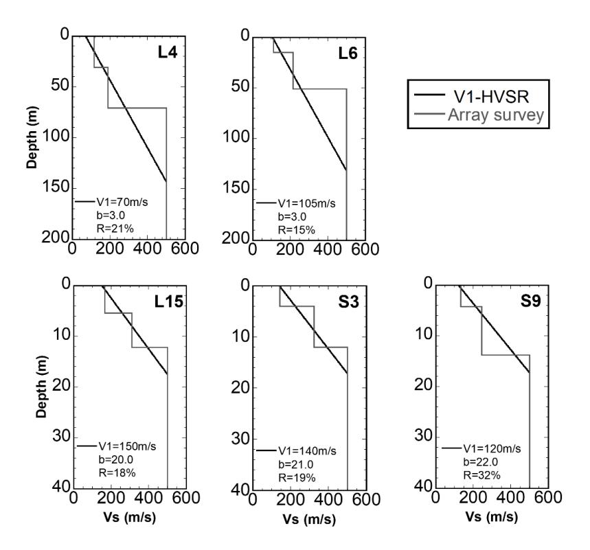
Figure 10 The Vs profiles of the V1-HVSR measurements are represented by black lines, and the estimated Vs profiles from a previous microtremor array survey [53] are represented by gray lines at five sites in the Bandung Basin. V1 and gradient (b) of Vs profile using the proposed method are shown for each site. The R-value of each profile comparison is shown in each plot.
5 Comparison with Results from Microtremor Array Survey
5.1 Comparison with Observed Phase Velocities from Microtremor Array Survey
The reliability of the estimated Vs profiles was investigated by comparison of the observed Rayleigh wave phase velocities from a previous microtremor array survey [53]. It is noted that the phase velocities in [53] were obtained from microtremor data at arrays with sizes of more than 10 m. This is sufficient to retrieve Rayleigh wave phase velocities in wider frequency ranges than the active seismic measurements in this study. We calculated the theoretical phase velocities for the fundamental mode of Rayleigh waves in our Vs profiles to compare them with the observed phase velocities, as shown in Figure 11. The phase velocity comparison at L4 revealed that the theoretical phase velocity of our Vs profile was well-matched with those observed at frequencies lower than 3 Hz and was somewhat similar at frequencies of 3 to 10 Hz. We also see in the phase velocity comparison at L6 that the theoretical phase velocity of our Vs profile agreed well with the observed phase velocity at frequencies higher than 3 Hz and had a similar trend at frequencies lower than 3 Hz. The theoretical phase velocities of the estimated Vs profiles at L15 and S3 had similar features to those observed at frequencies of 10 to 18 Hz at L15 and at frequencies of 10 to 17 Hz at S3. However, the observed phase velocities at L15 and S3 were lower than the theoretical ones at frequencies higher than 18 Hz. Moreover, the comparison of the phase velocity at S9 shows that the theoretical phase velocity of the estimated Vs profile was slightly higher than the observed phase velocity in the entire range of frequencies, even though the estimated V1 was similar to the observed phase velocity at high frequency. It is noted that the site of the V1- HVSR measurement at S9 was located at a distance of a 40 m apart from the location of the site in the previous array survey because of new construction around the original site. Therefore, the difference in phase velocities may have been caused by near-surface variation of the S-wave velocities at the two locations. As a confirmation for the phase velocity comparison, the Vs profile comparisons between the present and the previous study are shown in Figure 10. We observe that the layers above a bedrock of the Vs profiles in the previous study were well-approximated by the estimated Vs profiles. The Rvalues also show around and less than 20%, except at the S9 site, which is consistent with the results in the phase velocity comparison.
From the phase velocity comparison, we confirmed the appropriateness of the approximation of the profiles with the linear function. Furthermore, the comparison also indicates the importance of a priori information such as observed phase velocities in a wide frequency range or borehole (P-S logging) data at representative sites in the investigated area to confirm the appropriateness of the profile representation using the linear function. If the assumption of a linear velocity representation cannot be sufficiently satisfied by observed phase velocities or borehole profiles, the proposed method cannot be easily applied in such an area.
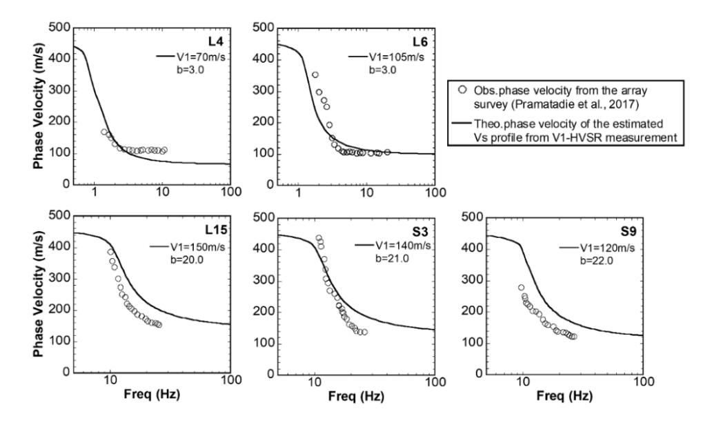
Figure 11 Comparison of phase velocity at five sites in Bandung Basin (See Figure 2 for the site locations). Circles and solid black lines indicate observed phase velocities from the microtremor array surveys [53] and the theoretical phase velocities of the estimated Vs profiles from the V1-HVSR measurements, respectively. VI and b of the estimated Vs profiles for the theoretical phase velocity are shown for each site.
5.2 Comparison of Vs30
Here, we compare the time-averaged S-wave velocities in the top 30 m (Vs30 in the following) of our Vs profiles with those of the Vs profiles from the microtremor array survey in [53], as shown in Table 3. The Vs30 has been frequently used as site classification for engineering purposes, such as the National Earthquake Hazards Reduction Program (NEHRP) site classification [57]. The value of Vs30 is calculated as follows:
\[Vs30 = \frac{30}{TT_{(0-30)}} = \frac{30}{\left(\sum_{i=1}^{n} \frac{d_i}{Vs_i}\right)}\] (5)
where \(TT_{(0.30)}\) is the travel time from the surface to a depth of 30 m. \(d_i\), \(Vs_i\), and n are the thickness and the S-wave velocity of the i-th layer, and the total number of layers to a depth of 30 m. In doing the computations of Vs30, we discretized our profile into numerous thin layers, each with a thickness of 0.1 m. We observed that the Vs30s of our profiles were approximately the same as those of the Vs profiles from the array survey. The Vs profiles estimated from the proposed method could adequately provide the Vs30s. However, a slightly higher Vs30 was observed in our profile of S9, which was caused by the different site-locations between the V1-HVSR measurement and the array survey.
Tabel 1 Comparison of the Vs30s of the estimated Vs profiles from V1-HVSR measurements with the Vs30s of the obtained Vs profiles from a microtremor array survey.
| Site | Vs30 of the Vs profile from the array survey in Pramatadie et al. [53] (m/s) | Vs30 of the estimated Vs profile from the V1-HVSR measurement (m/s) |
|---|---|---|
| L4 | 115 | 109 |
| L6 | 152 | 145 |
| L15 | 334 | 352 |
| S3 | 339 | 347 |
| S9 | 291 | 332 |
5.3 Comparison of Site Amplification Factors
We compared the 1D site amplification factors calculated for our Vs profiles with the Vs profiles estimated by Pramatadie et al. [53], as shown in Figure 12. The site amplification factor for vertically propagating S-waves was calculated using the same procedures as those in [53]. We assumed a constant Q-value of the S-waves as one-fifth of the S-wave velocity of each layer in meters per second.
The fundamental peak frequencies of the site amplifications from both profiles were similar. Moreover, we also saw a similarity in the amplification factors at frequencies of the fundamental peaks. Since the velocity contrast controls the peak amplitude of the amplification factors of a site [57,58], the similarity in the amplification factors of the two profiles was caused by the similarity in the contrast between the velocities of the bedrock and the top layers in our Vs profiles and those estimated by Pramatadie et al. [53]. This finding also indicates the advantageous usage of the linear velocity profile for estimating only the site fundamental peak frequency, as was done by Wang et al. [32], to obtain the site fundamental peak amplitude.
6 Influence of Different Bedrock Velocity
Since we assumed a given bedrock velocity (VB) in the proposed method, we also investigated the effect of various VB values on the estimated the Vs profiles in the Bandung Basin. Figure 13 compares the results of the estimated Vs
profiles with an assumed VB of 500 m/s, 600 m/s, and 700 m/s. The gradients of the estimated Vs profiles differed slightly from each other. Since the peak frequency of the theoretical ellipticity to determine the gradient is controlled by the ratio of the average velocity to the thickness of the surface layers [59], the variation of the VB could cause a change in the average velocity of the estimated Vs profile. Consequently, the gradients must be adjusted to produce a peak frequency similar to that of the theoretical ellipticity. Therefore, we found slight differences in the estimated gradients when changing the value of VB.
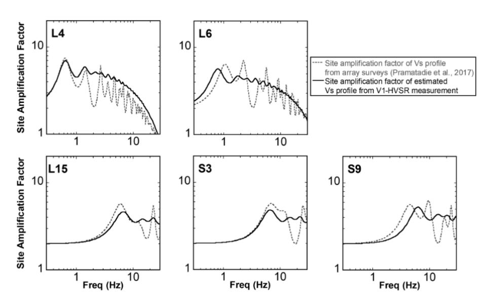
Figure 12 Site amplification factors at five sites in the Bandung Basin. Dashed gray and solid black lines represent the site amplification factors from the Vs profiles from Pramatadie et al. [53] and the estimated Vs profiles in this study, respectively.
We could obtain a profile with a deep bedrock depth by increasing VB, as found in the results of L4, L6, and L15. However, we observed that the estimated profile using VB of 600 m/s at S3 had a similar bedrock depth as the profile estimated using VB of 700 m/s. Moreover, the bedrock depth of the estimated profile using a VB of 500 m/s at S3 was much lower than the estimated profile using other VBs. To confirm the reasons for these unique results, we compared the theoretical ellipticities of the estimated profile using various VBs in Figure 14. The sharp peaks of the theoretical ellipticities did not appear for VBs of 500 m/ and 600 m/s at this site because the estimated profiles had a low velocity contrast between the velocities of the surface and the bedrock layers. Moreover, a profile with a low velocity contrast has a slight deviation in the peak frequency of the ellipticity [60]. Therefore, slight changes in the estimated
gradients with different VBs were observed in the results from S3. Since the peak frequency of the theoretical ellipticity is not dominant for a profile with low velocity contrast, we cannot apply the proposed method if the peak frequency of the ellipticity is difficult to identify. Moreover, the estimation of an accurate bedrock depth is not one of the general features of the proposed method.
We further evaluated the effects of different values of VBs by comparing the R values of the estimated Vs profiles in Table 4. The R values for the estimated Vs profiles with a VB of 600 m/s, and 700 m/s were calculated to compare the profile with a VB of 500 m/s. We observed that an increase of the VBs caused an increase of R. The largest R was found for S9 with values of 15% and 24% for the Vs profiles, with an assumed VBs of 600 m/s and 700 m/s, respectively. The estimated Vs profiles with different VBs had R values less than 20%, indicating a relatively good agreement with the Vs profile with the proper VB.
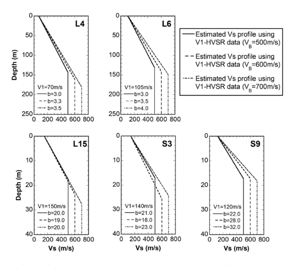
Figure 13 Comparison of the estimated Vs profiles using different bedrock velocities at five sites in the Bandung Basin. The estimated Vs profiles with
assumed bedrock velocities of 500 m/s, 600 m/s, and 700 m/s correspond to the solid black, dashed, and dash-dotted lines, respectively. The R values of each estimated Vs profile are listed in Table 4.
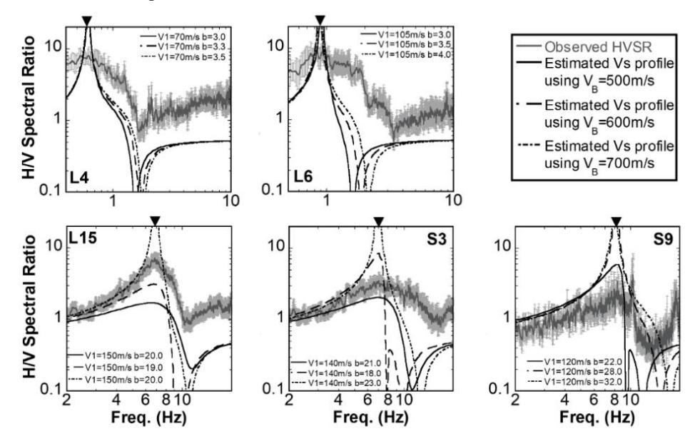
Figure 14 Comparison of the theoretical ellipticities of the estimated profiles using different bedrock velocities at five sites in the Bandung Basin. Solid, dashed, and dash-dotted black lines indicate the theoretical ellipticities of the fundamental mode Rayleigh wave of the profiles with assumed bedrock velocities of 500 m/s, 600 m/s, and 700 m/s, respectively. Solid gray and light gray lines represent the observed HVSRs with standard deviation. The black inverted triangles indicate the peak frequencies of the observed HVSR.
Tabel 2 List of R-values for estimated Vs profiles from V1-HVSR measurements using different bedrock velocities.
| Site | R value relative to estimated Vs profile based on V1-HVSR data with VB = 500m/s | ||||
|---|---|---|---|---|---|
| VB = 600m/s | VB = 700m/s | ||||
| L4 | 7% | 11% | |||
| L6 | 10% | 19% | |||
| L15 | 2% | 0% | |||
| S3 | 7% | 5% | |||
| S9 | 15% | 24% | |||
7 Conclusions
We proposed a method for 1D S-wave velocity profile estimation using observed surface S-wave velocity (V1) and peak frequency of the microtremor HVSR. The 1D Vs profile is presented with a linear velocity function over a bedrock with a given velocity. This reduces the number of the model parameters to two: V1 and velocity gradient. Since V1 can be derived from field measurements, the profile is uniquely estimated by a determination of the gradient from the agreement of the peak frequencies between the observed HVSR and the theoretical ellipticity of the Rayleigh wave.
The applicability of the proposed method was confirmed by numerical tests. The profiles from the boreholes were well-reconstructed with synthetic observed data. We also applied the proposed method to actual data from five sites in the Bandung Basin, Indonesia. We performed short-length active seismic wave measurements for V1 and single three-component microtremor measurements for the HVSR at each site, respectively. We could easily determine the velocity gradient with a one-dimensional grid search procedure using the measured V1 and the peak frequency of the observed HVSRs. The appropriateness of the estimated Vs profiles based on the proposed method was confirmed by comparison of the theoretical phase velocities for the estimated Vs profiles with the Rayleigh-wave phase velocities observed in a previous microtremor array survey.
The proposed method has limitations in terms of the estimation of bedrock depths and the accommodation of complex configurations of sediments with different velocity gradients. However, Vs profiles from this method can provide accurate peak frequencies and amplification factors for site amplification, because the peak frequency of the observed HVSR and the velocity contrast between the surface and the bedrock are inherently reconstructed in the profile. Hence, the proposed method is suitable for providing Vs profiles for site effect evaluation, and the fundamental peaks of site amplification factors with easier data acquisition and a simpler procedure for profile estimation than the existing standard methods. However, the assumption of a linear profile representation used in the proposed method may be difficult to apply if a profile contains layers with high velocity contrast, or has a thick layer with a constant velocity, or an inverse velocity layer. Therefore, we recommend that the appropriateness of the linear S-wave velocity profile representation in the investigated area must first be confirmed from observed phase velocities in a wide frequency range or from borehole profiles at representative sites before usage of the proposed method.
Acknowledgments
We wish to express our thanks to all reviewers and editors for their comments, which helped to improve this manuscript. We gratefully acknowledge K. Ishige and S. Shimizu at Tokyo Institute of Technology, and M. Sabila Rasyad and S. Aisyah at Institut Teknologi Bandung for their support in doing the field measurements. We are also grateful to Dr. Kosuke Chimoto at Kagawa University for his helpful discussions during this research. We thank the Ministry of Education, Culture, Sports, Science and Technology (MEXT), Japan for their scholarship, and the Consortium for Socio-Functional Continuity Technology Project (SOFTech) for their financial support of the first author during a doctoral program at Tokyo Institute of Technology. We also thank to LPPM Hasanuddin University (00323/UN4.22/PT.01.03/2023) for its financial support.