
1 Introduction
The consumption of cashew nuts in the world market is growing yearly because of their widely appreciated taste and high nutrient content [1]-[3]. Frequent consumption of cashew nuts minimizes cholesterol, hypertension, coronary heart disease, and diabetes [4],[5]. Furthermore, the cashew nut is a cash product in most countries where it is grown, increasing the foreign exchange earnings for the nation and as a source of income for most families [6].
The cashew nut is cultivated worldwide. Africa contributes about 40% of worldwide production, while Tanzania generates roughly 20% of all African production [7]. More than 80% of the total output in Tanzania comes from the Lindi and Mtwara regions [8]. Cashew nuts are the main cash crop for many families in the southern regions and contribute up to 10% of the total value of earnings in foreign currencies [9].
Received September 22nd, 2022, Revised June 1 st, 2023, Accepted for publication July 4 th, 2023 Copyright © 2023 Published by ITB Institute for Research and Community Service, ISSN: 2337-5760, DOI: 10.5614/j.math.fund.sci.2023.55.1.3
Despite the significant contribution to the nation and the continent, cashew nut production has been impacted by numerous issues, such as diseases, declining soil fertility, drought, and insect pests [10],[11]. Cashew Fusarium wilt disease destroys many cashew plants in Tanzania, which is where the disease was first discovered [12]. The disease is caused by a soil-borne fungus called Fusarium oxysporum [12]-[14]. As a result of this disease's ability to damage cashew plants, households and the nation's overall cashew production and income are reduced [12],[15].
Fusarium wilt disease outbreaks have been experienced in the south-eastern part of Tanzania, including the Mtwara Rural, Newala, Masasi and Tandahimba districts in the Mtwara region and Liwale, Nachingwea and Ruangwa districts in the Lindi region [15]. The main transmission of Fusarium wilt disease is through root contact [16]. Dead infected cashew plants contribute to disease transmission [17]. The fungus in diseased-induced dead cashew plants invades the plant tissue and produces macroconidia. After the host tissue has degraded, chlamydospores are produced and end up in the soil when the tissue collapses [18]. This is possible when disease-induced dead plants are left to decompose in the field. Farmers usually leave the dead plants to deteriorate in the field, as indicated in Figure 1.
Figure 1 Photograph of disease-induced dead cashew plant. Source: Field data, 2020.
Mathematical modelling is essential for understanding disease dynamics and suggesting appropriate control methods for minimizing infectious diseases [19]- [24]. Plant disease dynamics can be modelled mathematically, as has been shown in different studies. For example, Burie et al. [25] investigated vineyard fungal disease through a mathematical model and devised short and long-term solutions. Anggriani [26] analyzed plant-fungal epidemics and ended up with remedial
factors against infection. Nisar et al. [27] modelled the Gemini virus in capsicum annuum and developed the best strategy for eliminating the disease at an affordable cost.
Additionally, mathematical modelling assists decision-makers in deciding on the most effective control strategies by using the information from a sensitivity analysis that identifies the parameters that contribute to the spread of the disease [28]-[32].
This study applied mathematical theories in modelling the role of decomposed disease-induced dead cashew plants in disease transmission and persistence during an outbreak. The findings can help to develop strategies for disease management and understanding how the disease develops and spreads over time.
2 Model Formulation
This section deals with the model formulation whereby cashew plants are divided into five subpopulations. The susceptible plant (P) is a cashew plant that is disease-free yet prone to infection when the fungus comes into contact with it. The plants become exposed (E) after touching diseased plants or contaminated soil through its wounds or roots [14],[33]-[36]. After two to six months, the exposed population becomes infectious (W). The infectious population can either be treated and join the treated population (T) or die due to disease and join the dead class (D) [15]. Also, there are two subgroups of the fungal population, i.e., macroconidia spores (M) and chlamydospores (H). Macroconidia spores occur on the exterior of disease-induced dead plants. Macroconidia spores on the surface of disease-induced dead plants produce chlamydospores and fall to the ground [13],[37].
The model was developed assuming that the population growth of cashew plants follows a logistic behavior, where r is the growth rate and \(k_1\) is the carrying capacity. The contact rate between fungus and plants is modelled by \(\beta\) with the infection rate expressed as follows:
\[\beta = \left(\frac{\tau_1 H}{d + H} + \tau_2 W\right). \tag{1}\]
The parameter \(\tau_1\) represents the contact rate between vulnerable cashew plants and chlamydospores, while \(\tau_2\) is the contact rate between susceptible cashew
plants and diseased plants [14]. The parameter d denotes the ground-level chlamydospore saturation constant rate. The parameter represents the progression rate of the exposed population to the infected population within two to six months [18]. Cashew plants that are not seriously infected may regain health after treatment at rate and develop susceptibility with rate [15]. Cashew plants that are more seriously impacted have a lower survival rate and perish at a rate of , or die naturally at a rate of [15]. Usually, farmers remove some dead plants from the field for other uses while some dead plants remain to decompose in the field, denoted by . Microconidia spores attack the tissue of dying plants to produce macroconidia spores from the sporodochia [37]-[42]. The parameter defines the rate at which exposed, infected, and disease-induced dead plants produce macroconidia spores. The following equation represents this parameter:
\[\psi = \upsilon E + \gamma W + \pi D. \tag{2}\]
Macroconidia produce chlamydospores at rate [43]-[45]. Chlamydospores are thick-walled, which helps them to survive in an unfavorable environment for a long time [46]. Chlamydospores leave the living class due to deterioration at rate [13].
2.1 Parameter Descriptions
Based on the description of the dynamics of Fusarium wilt disease and the assumptions, the compartmental diagram in Figure 2 captures the constructed interaction between cashew plants and Fusarium oxysporum fungus.
Figure 2 Compartment flow diagram.
The model parameters used are summarized in Table 1.
Table 1 Parameters and their description for Fusarium wilt disease
| Symbol | Description |
|---|---|
| r | Cashew plant's growth rate |
| \(\tau_1\) | Contact rate between susceptible cashew plants and chlamydospores |
| \(\tau_2\) | Contact rate between susceptible and infected cashew plants |
| \(k_{1}\) | Carrying capacity of cashew plants |
| d | Chlamydospores saturation in the soil |
| \(\omega\) | Rate of progression from exposed population to infected population |
| \(\alpha\) | Rate of natural death |
| \(\theta\) | Disease-related mortality rate |
| ν | Disease-induced dead plants left to decompose in the field |
| \(\phi\) | Rate at which recovered plants return to the susceptible class |
| \(\upsilon\) | Production rate of macroconidia from dead exposed plants |
| γ | Production rate of macroconidia from dead infected plants |
| \(\pi\) | Production rate of macroconidia from disease-induced dead plants |
| \(\eta\) | Production rate of chlamydospores |
| \(\mu\) | Decay rate of chlamydospores |
2.2 Mathematical Equations
Considering the flow diagram, we developed mathematical equations that show the transmission dynamics of the Fusarium wilt disease using the ordinary differential equation:
\[\frac{dP}{dt} = rP\left(1 - \frac{P}{k_1}\right) + \phi T - \left(\frac{\tau_1 H}{d + H} + \tau_2 W\right) P\] \[\frac{dE}{dt} = \left(\frac{\tau_1 H}{d + H} + \tau_2 W\right) P - (\alpha + \omega) E\] \[\frac{dW}{dt} = \omega E - (\alpha + \rho + \theta) W\] \[\frac{dT}{dt} = \rho W - (\alpha + \phi) T\] (3)
\[\frac{dD}{dt} = \theta W - vD\] \[\frac{dM}{dt} = vE + \gamma W + \pi D - \eta M\] \[\frac{dH}{dt} = \eta M - \mu H\]
3 Qualitative Analysis
A qualitative analysis of the model was conducted to gain insight into the dynamical characteristics of model (3) and to better comprehend the effects of the presence of decomposed plants.
3.1 Non-negativity of the Solution
It must be demonstrated that all system solutions with positive initial values remain positive for model system (3) to be epidemiologically significant and adequately posed. The following theorem will prove this.
Theorem 3.1
Assume that P(0) > 0, E(0) > 0, W(0) > 0, T(0) > 0, D(0) > 0, M(0) > 0 and H(0) > 0. Then, the solutions P(t), E(t), W(t), T(t), D(t), M(t), H(t) of model (3) are positive \(\forall t > 0\).
Proof. Consider the first equation in model (3) that forms the following inequality:
\[\frac{dP(t)}{P(t)} \ge -\left(\frac{\tau_2 H(t)}{d + H(t)} + \tau_1 W(t)\right) dt.\]
Solving for t and P(t) = P(0), we get:
\[P(t) \ge P(0)e^{-\int_0^t \left(\frac{\tau_2 H(t)}{d+H(t)} + \tau_1 W(t)\right) dt}.\]
As \[t \to \infty\], the value of \(P(t) \ge P(0)e^{-\int\limits_0^t \left(\frac{\tau_2 H(t)}{d+H(t)} + \tau_1 W(t)\right)dt} \ge 0\), since
\[\frac{\tau_2 H(t)}{d + H(t)} + \tau_1 W(t) \ge 0.\]
A similar proof can be established for the remaining equation in the \(\mathfrak{R}^7_+\) region and the system can be used to research cashew disease since it is meaningful.
3.2 Existence and Uniqueness of the Solution
Considering the general form of ordinary first-order differential equations,
\[\frac{dy}{dt} = f(t, y) \tag{4}\] where the initial value \(t_0\) with respect to the function can be written as \(y(t_0) = y_0\).
The following theorem shows the existence of a unique solution of the Fusarium wilt disease model.
Theorem 3, 2
Assume there exists a domain D such that:
\[\left|t - t_0\right| \le p \left|y - y_0\right| \le q,\tag{5}\] and if g(t, y) satisfies the Lipschitz condition such that:
\[||G(t, y_1) - G(t, y_2)|| \le b ||y_1 - y_2||\] (6)
where G is a function and at any time point \((t, y_1) \in D\) and \((t, y_2) \in D\), the parameter b represents a positive constant. Then, there is a constant \(\varepsilon > 0\) such that \(\exists\) is a continuous solution y(t) of system (1) such that \(|t - t_0| \le \varepsilon\). The system should also satisfy the following condition:
\[\frac{\partial G_i}{\partial y_j}, i, j = 1, 2, 3, \dots n \tag{7}\]
It is bounded and continuous within the domain D.
Lemma 3. 1 If G(t, y) is a continuous partial derivative \(\frac{\partial G_i}{\partial y_i}\) on a bounded and closed convex domain D that satisfies the Lipschitz condition. Hence, we need to find a fixed solution to the following form:
\[0 < D < \infty \tag{8}\]
Theorem 3.3 Assume that the domain D satisfies conditions (6) and (7) in theorem 3.2. Then a mathematical solution to model (3) is bounded in domain D.
Proof. The proof of theorem 3.3 is obtained by considering lemma 3.1. Consider the following equations:
\[G_{1} = rP\left(1 - \frac{P}{k_{1}}\right) + \phi T - \left(\frac{\tau_{1}H}{d+H} + \tau_{2}W\right)P\] \[G_{2} = \left(\frac{\tau_{1}H}{d+H} + \tau_{2}W\right)P - (\alpha + \omega)E\] \[G_{3} = \omega E - (\alpha + \rho + \theta)W\] \[G_{4} = \rho W - (\alpha + \phi)T\] \[G_{5} = \theta W - \nu D\] \[G_{6} = \nu E + \gamma W + \pi D - \eta M\] \[G_{7} = \eta M - \mu H\] \[(9)\]
We need to show that \(\frac{\partial G_i}{\partial y_j}\), j=1,2,....7 are bounded and continuous. The following are the partial derivatives of model (9) for a unique equation. Considering the first equation in model (9), we have:
\[G_{1} = rP\left(1 - \frac{P}{k_{1}}\right) + \phi T - \left(\frac{\tau_{1}H}{d+H} + \tau_{2}W\right)P.\]
The partial derivative of function \(G_1\) with respect to class P is:
\[\frac{\partial G_1}{\partial P} = r \left( 1 - \frac{P}{k_1} \right) - \frac{\tau_1 H}{d + H} - \tau_2 W .\]
Take the absolute value of both sides by considering condition (8), we get:
\[\left| \frac{\partial G_1}{\partial P} \right| = \left| r \left( 1 - \frac{P}{k_1} \right) - \frac{\tau_1 H}{d + H} - \tau_2 W \right| < \infty.\]
Then finding the partial derivative of function \(G_1\) with respect to class W gives:
\[\frac{\partial G_1}{\partial W} = -\tau_2 P\] thus \(\left| \frac{\partial G_1}{\partial W} \right| = \left| -\tau_2 P \right| < \infty\).
Also, the partial derivative of function \(G_{\scriptscriptstyle 1}\) with respect to class T gives:
\[\frac{\partial G_1}{\partial T} = \varphi\], then \(\left| \frac{\partial G_1}{\partial T} \right| = \left| \varphi \right| < \infty\).
Lastly, find the partial derivative of function \(G_1\) with respect to class H gives:
\[\frac{\partial G_1}{\partial H} = -S\left(-\frac{\tau_1 H}{\left(d+H\right)^2} + \frac{\tau_1}{d+H}\right).\]
With condition (6), we have:
\[\left|\frac{\partial G_1}{\partial H}\right| = \left|-P\left(-\frac{\tau_1 H}{\left(d+H\right)^2} + \frac{\tau_1}{d+H}\right)\right| < \infty.\]
Then, consider the second equation in model system (8). We have:
\[G_2 = \left(\frac{\tau_1 H}{d + H} + \tau_2 W\right) P - (\alpha + \omega) E.\]
Its partial derivative with respect to class P is as follows:
\[\frac{\partial G_2}{\partial P} = \frac{\tau_1 H}{d+H} + \tau_2 W \text{, thus } \left| \frac{\partial G_2}{\partial P} \right| = \left| \frac{\tau_1 H}{d+H} + \tau_2 W \right| < \infty.\]
The partial derivative of function \(G_2\) with respect to class E is as follows:
\[\frac{\partial G_2}{\partial F} = -\alpha - \omega.\]
By considering condition (7), we get:
\[\left|\frac{\partial G_2}{\partial E}\right| = \left|-\alpha - \omega\right| < \infty.\]
Again, the partial derivative of function \(G_2\) with respect to class W is as follows:
\[\frac{\partial G_2}{\partial W} = \tau_2 P\]
Taking the absolute value, we get:
\[\left|\frac{\partial G_2}{\partial W}\right| = \left|\tau_2 P\right| < \infty.\]
The remaining equations in model system (9) should be solved using a similar methodology. This demonstrates that every partial derivative is continuous and bounded. Hence, this proves the existence and uniqueness of the solution of system (3) in region D.
3.3 Fusarium Wilt Equilibria
The Fusarium wilt disease-free equilibrium point \((E_0)\) is given by:
\[E_0 = (k_1, 0, 0, 0, 0, 0, 0)\]
And the endemic equilibrium points \((E_*)\) are:
And the endemic equinorium points \[(E_*)\] are. \[P^* = \frac{\alpha \left(\alpha + \omega\right) W^*}{\left(\frac{\tau_1}{d} + \tau_2 W^*\right) \omega}, \ E^* = \frac{\alpha W^*}{\omega}, \ T^* = \frac{\rho W^*}{\alpha + \phi}, \ D^* = \frac{\theta W^*}{\nu}, \ H^* = \frac{\eta M^*}{\mu}\] and \[M^* = \frac{\left(\gamma + \frac{\pi \theta}{\nu} + \frac{\alpha \nu}{\omega}\right)}{\eta} W^*.\]
3.4 Reproduction Number Analysis
The basic reproduction number \(\Re_0\) was used to investigate the local and global stability of model system (3). The calculation of \(\Re_0\) was done by using the next-generation operation method in [47].
\[F = \begin{bmatrix} \left(\frac{\tau_1 H}{d+H} + \tau_2 W\right) P \\ 0 \\ 0 \\ 0 \\ 0 \end{bmatrix} \text{ and } V = \begin{bmatrix} (\alpha + \omega) E \\ \omega E - (\alpha + \rho + \theta) W \\ \theta W - \nu D \\ \nu E + \gamma W + \pi D - \eta M \\ \eta M - \mu H \end{bmatrix}\](10)
Assume matrix F(x) is the Jacobian matrix from F and V(x) is the Jacobian matrix from V. The matrices F(x) and V(x) at disease-free equilibrium \(E_0 = (k_1, 0, 0, 0, 0, 0, 0)\) obtained are:
\[\text{[rumus tidak dapat ditampilkan dengan baik — lihat PDF asli]}\]
The next-generation matrix obtained is:
\[\text{[rumus tidak dapat ditampilkan dengan baik — lihat PDF asli]}\]
\[\text{[rumus tidak dapat ditampilkan dengan baik — lihat PDF asli]}\]
The eigenvalues obtained are:
\[\lambda_{1} = 0, \lambda_{2} = 0, \lambda_{3} = 0, \lambda_{4} = 0, \lambda_{5} = \frac{k_{1}\omega\tau_{1}}{(\alpha + \theta + \rho)(\alpha + \omega)} + \frac{k_{1}\tau_{2}\left(\nu\upsilon(\alpha + \theta + \rho) + \omega(\pi\theta + \gamma\nu)\right)}{d\,\mu\nu(\alpha + \theta + \rho)(\alpha + \omega)}\]
The reproductive number is the absolute largest eigenvalue obtained, which is:
\[\mathfrak{R}_{0} = \frac{k_{1}\omega\tau_{1}}{(\alpha+\theta+\rho)(\alpha+\omega)} + \frac{k_{1}\tau_{2}\left(\nu\upsilon(\alpha+\theta+\rho)+\omega(\pi\theta+\gamma\nu)\right)}{d\mu\nu(\alpha+\theta+\rho)(\alpha+\omega)}.\] (15)
The basic reproduction number represents the projected number of each plant infected by the initially diseased plants for their whole infectious period. It serves as a predictor of the ability of infectious and parasitic organisms to spread.
3.5 Local Stability
A stability study of the disease-free equilibrium point of model system (3) was conducted using the Routh-Hurwitz criterion [48]. Consider Theorem 3.4 below.
Theorem 3.4
The Fusarium wilt disease-free equilibrium point is locally asymptotically stable if and only if the major diagonal of the Jacobian matrix is positive.
Proof. Assume that each equation in the system is differentiated, considering its state variable at \(E_0\). The Jacobian matrix at \(E_0\) is as follows:
\[J_{E_0} = \begin{bmatrix} -r & k_1 \tau_2 & 0 & \varphi & 0 & 0 & \frac{-k_1 \tau_1}{d} \\ 0 & -(\alpha + \omega) & k_1 \tau_2 & 0 & 0 & 0 & \frac{k_1 \tau_1}{d} \\ 0 & \omega & -(\alpha + \theta + \rho) & 0 & 0 & 0 & 0 \\ 0 & 0 & \rho & -(\alpha + \phi) & 0 & 0 & 0 \\ 0 & 0 & \theta & 0 & -\nu & 0 & 0 \\ 0 & \nu & \gamma & 0 & \pi & -\eta & 0 \\ 0 & 0 & 0 & 0 & 0 & \eta & -\mu \end{bmatrix}\](16)
Computing the eigenvalues of the Jacobian matrix \(J_{E_0}\), we obtain -r and \(-(\alpha + \phi)\). Then the remaining eigenvalues will be obtained from matrix H below.
\[H = \begin{bmatrix} A_{ij} \end{bmatrix} = \begin{bmatrix} -(\alpha + \omega) & k_1 \tau_2 & 0 & 0 & \frac{k_1 \tau_1}{d} \\ \omega & -(\alpha + \theta + \rho) & 0 & 0 & 0 \\ 0 & \theta & -\nu & 0 & 0 \\ \nu & \gamma & \pi & -\eta & 0 \\ 0 & 0 & 0 & \eta & -\mu \end{bmatrix}\](17)
To obtain the remaining eigenvalues, we consider the polynomial roots \(|H - \lambda| = 0\) that give the characteristic equation (18):
\[\lambda^{5} + c_{1}\lambda^{4} + c_{2}\lambda^{3} + c_{3}\lambda^{2} + c_{4}\lambda + c_{5} = 0.\] where: \[c_{1} = \mu + \eta + \nu + 2\alpha + \theta + \rho + \omega\] \[c_{2} = \alpha^{2} + 2\alpha(\eta + \mu + \nu) + \alpha(\omega + \rho + \theta) + \eta(\mu + \nu) + \omega(\mu + \nu + \omega + \rho + \theta) + \mu(\nu + \omega + \rho + \theta) + \nu(\omega + \rho) - \omega k_{1}\tau_{2}\] \[\text{[rumus tidak dapat ditampilkan dengan baik — lihat PDF asli]}\]
The positivity of the principal leading diagonal of matrix \(H_n\) makes the disease-free equilibrium point locally stable. In light of this, the disease-free equilibrium point is only locally stable when \(\Delta H_1\), \(\Delta H_2\),... \(\Delta H_5 > 0\). Then, \(\Delta H_1 > 0\) since we have
\[\mu + \eta + \nu + 2\alpha + \theta + \rho + \omega > 0\]
\[\mu + \eta + \nu + 2\alpha + \theta + \rho + \omega > 0\] Then, for \(\Delta H_2 > 0\), if and only if \(c_1c_2 > c_3\), \(\Delta H_3 > 0\), if \(c_1c_2c_3 + c_3^2 > c_1c_4 + c_5\), \(\Delta H_4 > 0\) if \(c_1c_2c_3c_4 + c_2c_3c_5 + c_5^2 > c_2c_5 + c_1^2c_4^2 + c_3^2c_4^2\), and lastly \(\Delta H_5 > 0\) if \(c_1c_2c_3c_4c_5 + c_1^2c_4^2c_5 + c_1c_4c_5^2 > c_1c_2^2c_5^2\).
Since the principal leading diagonal of the Jacobean matrix is all positive, the disease-free equilibrium point \(E_0\) is locally asymptotically stable.
3.6 Global Stability
The following theorem is presented to comprehend the disease-free equilibrium's global stability.
Theorem 3.5. If \(\Re_0 < 1\), the disease-free equilibrium is globally asymptotically stable, and unstable otherwise.
Proof. Apply the comparison theorem [49] to ascertain global stability while accounting for the derivatives of the diseased compartments in model system (3).
\[\text{[rumus tidak dapat ditampilkan dengan baik — lihat PDF asli]}\]
\[\begin{pmatrix} \frac{dE}{dt} \\ \frac{dW}{dt} \\ \frac{dD}{dt} \\ \frac{dM}{dt} \\ \frac{dH}{dt} \end{pmatrix} \le (F - V) \begin{pmatrix} E \\ W \\ D \\ M \\ H \end{pmatrix}\] (20)
The matrices F and V presented in equations (19) and (20) are the following Jacobian matrices:
\[\text{[rumus tidak dapat ditampilkan dengan baik — lihat PDF asli]}\] and
\[V = \begin{pmatrix} \alpha + \omega & 0 & 0 & 0 & 0 \\ -\omega & \alpha + \rho + \theta & 0 & 0 & 0 \\ 0 & -\theta & \nu & 0 & 0 \\ -\upsilon & -\gamma & -\pi & \eta & 0 \\ 0 & 0 & 0 & -\eta & \mu \end{pmatrix}.\] (22)
Since the eigenvalues of matrix (F-V) have a negative real part, model (3) is stable at any time \(\Re_0 < 1\). Then \((P, E, W, T, D, M, H) \rightarrow (P^0, 0, 0, 0, 0, 0, 0, 0, 0)\) and \(P \rightarrow P^0\) as \(t \rightarrow \infty\). Considering the comparison theorem, we have \((P, E, W, T, D, M, H) \rightarrow E_0\) as \(t \rightarrow \infty\). Therefore, the disease-free equilibrium is globally asymptotically stable.
4 Data Presentation and Parameter Estimation
Ward extension staff, the district agriculture offices, and the Naliendele Agriculture Research Institution in Mtwara participated in the survey for data collection. The maximum likelihood method was used to fit and estimate the model parameters. The data for model fitting was obtained in the Lindi and Mtwara regions specifically.
4.1 Data Presentation
The most crucial components of modelling are model fitting and parameter estimation. After developing a mathematical model and collecting data for the desired class, one is well-positioned to fit the data into the model and determine its parameters [50]. The collected data based on cashew plant death due to Fusarium wilt disease came from seven districts in the Lindi and Mtwara regions in Tanzania. The districts where research was conducted included Tandahimba, Masasi, Newala and Mtwara Rural in the Mtwara region, while in the Lindi region, Liwale, Ruangwa and Lindi Rural were involved. The collected data was used in model parameter estimation. A summary of the data is presented in Table 1.
Table 2 Infected dead cashew plants from the year 2018 to 2020.
| Village Serial number | Village | Number of disease-induced dead plants | Village serial number | Village | Number of disease induced dead plants |
|---|---|---|---|---|---|
| 1 | Kitandi | 15 | 15 | Kitangali | 50 |
| 2 | Chinongwe | 45 | 16 | Chikunja | 30 |
| 3 | Ruhokwe | 46 | 17 | Msikisi | 16 |
| 4 | Simana | 23 | 16 | Makululu | 15 |
| 5 | Tuungane B | 56 | 19 | Mnavila | 17 |
| 6 | Tuungane A | 11 | 20 | Makong'on da | 41 |
| 7 | Ungongolo Sokoni | 24 | 21 | Lukuledi | 48 |
| 8 | Majimaji | 40 | 22 | Mchauru | 7 |
| 9 | Legeza mwendo | 15 | 23 | Mpindimbi | 9 |
| 10 | Itete | 50 | 24 | Namyomyo | 51 |
| 11 | Dihimba | 39 | 25 | Nangoo | 190 |
| 12 | Tandika | 31 | 26 | Nanganga | 204 |
| 13 | Mwera Sokoni | 13 | |||
| 14 | Nakayaka | 33 |
Source: Field data 2020
4.2 Estimation of Parameters And Model Fitting
The Matlab program was used to conduct a numerical simulation of model (1). The proposed model's parameter estimation and model fitting were done using maximum likelihood estimation (MLE), as described in [51]. Model fitting is essential since it determines the parameter values for a specific model system based on the data [26]. The initial parameter values, shown in Table 2, were generated from various publications, such as cashew plant carrying capacity k [52], the force of infection between chlamydospores fungus and susceptible plants [53], the force of infection between infected plants and susceptible plants [54], the saturation rate of fungus in the soil d [25], progression rate [18]. However, we assumed other parameter values based on epidemiological implications.
A graph of the model solution using data and values from the literature against time is shown in Table 1. The high deviation between the model solution and the data shown in Figure 3a indicates the necessity of parameter estimation. In comparison to Figure 3a, Figure 3b displays better results, and the solution of the model with the estimated parameters tends to follow the trend of the data. Table 2 shows the numerical values for each estimated parameter.
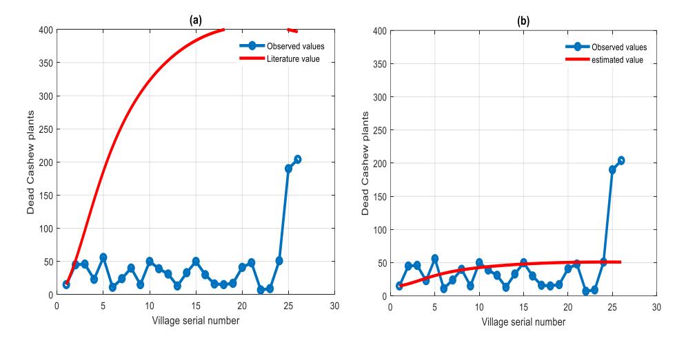
Figure 3 (a) Model solution with values from the literature that seems to diverge from the field data. (b) Fitting of the model solution with estimated values and field data that show convergence.
| Parameter | Literature value | Estimated value | Parameter | Literature value | Estimated |
|---|---|---|---|---|---|
| r | 0.05 | 0.0605 | \(\rho\) | 0.3 | 0.3757 |
| \(k_{\scriptscriptstyle 1}\) | 69 hector-1 | 74 hector-1 | \(\eta\) | 0.5 | 0.4784 |
| \(\tau_{_1}\) | 0.06 | 0.0608 | \(\mu\) | 0.05 | 0.0655 |
| \({\tau}_2\) | 0.0018 | 0.0016 | \(\nu\) | 0.05 | 0.0587 |
| d | 40 m-2 colony site density | 45.4016 | \(\phi\) | 0.3 | 0.3081 |
| \(\omega\) | 0.5 year | 0.4 | \(\boldsymbol{\nu}\) | 0.05 | 0.0481 |
| \(\alpha\) | 0.005 | 0.00038 | γ | 0.2 | 0.1968 |
| \(\theta\) | 0.8 | 0.093 | \(\pi\) | 0.4 | 0.4125 |
Table 3 Parameter values estimated and values from the literature.
5 Numerical Analysis
5.1 Local Sensitivity Analysis
This analysis gives indices that help determine how important each parameter is for Fusarium wilt disease transmission and incidence [55]. The local sensitivity analysis examines what happens to \(\mathfrak{R}_0\) when some parameters vary, employing the formula proposed by Arriola and Hyman [56]. Using sensitivity indices, we may evaluate how the state variable has changed relative to a parameter change. The normalized forward sensitivity index of a variable to a parameter measures how much the variable changes with a parameter [57]. The normalized forward sensitivity index is acquired when \(\mathfrak{R}_0\) is differentiable with respect to a given parameter, let's say \(\ell\), and can be computed as:
\[\Upsilon_q^{\mathfrak{R}_0} = \frac{\partial \mathfrak{R}_0}{\partial q} \times \frac{q}{\mathfrak{R}_0}.\]
The result is presented in Figure 4.
The output in Figure 4 indicates that the transmission rate of infection from the soil to vulnerable plants \(\tau_1\) and the decomposed disease-induced death rate \(\pi\) strongly influence disease transmission. Furthermore, if the treatment rate \(\rho\) and fungus decay rate \(\mu\) have negative indices, the increase in \(\rho\) and \(\mu\) will decrease disease transmission.
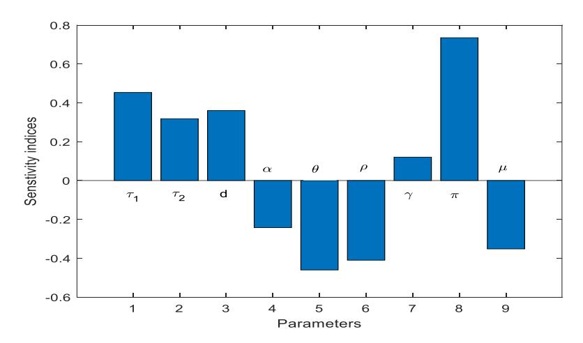
Figure 4 Local sensitivity analysis.
5.2 Global Sensitivity Analysis
The analysis was examined when all parameters were simultaneously varied across the entire range of each parameter. The results of this analysis, which was conducted using the partial rank correlation coefficient (PRCC) method, are shown in Figure 5. The results show that the decomposed disease-induced death rate and fungus saturation in the soil d increase the transmission of the disease. This means disease transmission increases as the values of the mentioned parameters decrease. Furthermore, disease transmission will decrease when the fungus decay rate , the number of dead plants remaining in the field , and the disease-induced death rate increase.
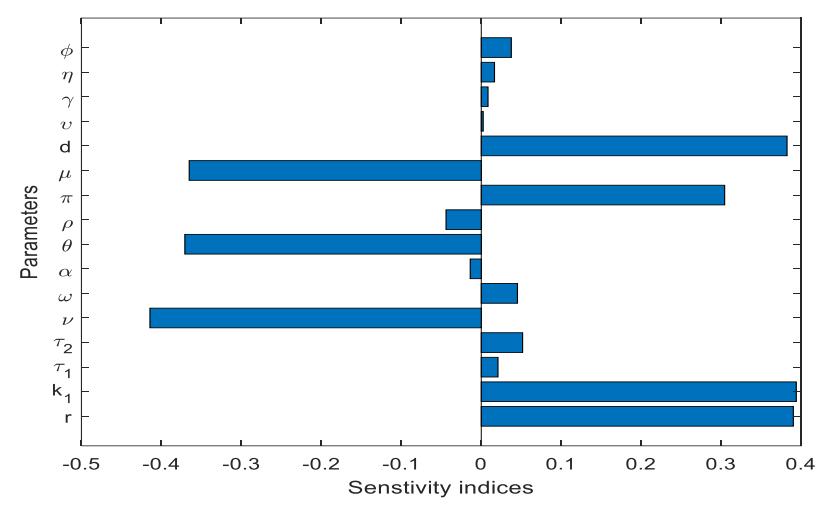
Figure 5 Global sensitivity analysis was conducted using the PRCC technique.
5.3 Effect of Decomposed Disease-Induced Dead Plants on Disease Transmission
Figures 6a, 6b and 6c show the contribution of decomposed disease-induced dead, infected, and exposed dead plants in producing macroconidia. Sporodochia from the dead infected plants produce macroconidia. Macroconidia spores are a saprophytic fungus that plays an important role in decomposition as it performs the initial steps [58],[59]. The growth rate of macroconidia increased in the first four months, as shown in Figures 6 a, b and c, due to the availability of food (dead plants). The growth rate from five to twenty months decreased as the decomposition rate increased. The increase in the macroconidia population led to a rise in disease transmission due to the increase in the chlamydospore population in the soil. Therefore, the presence of dead plants during an outbreak should be considered in planning and selecting a disease control method.
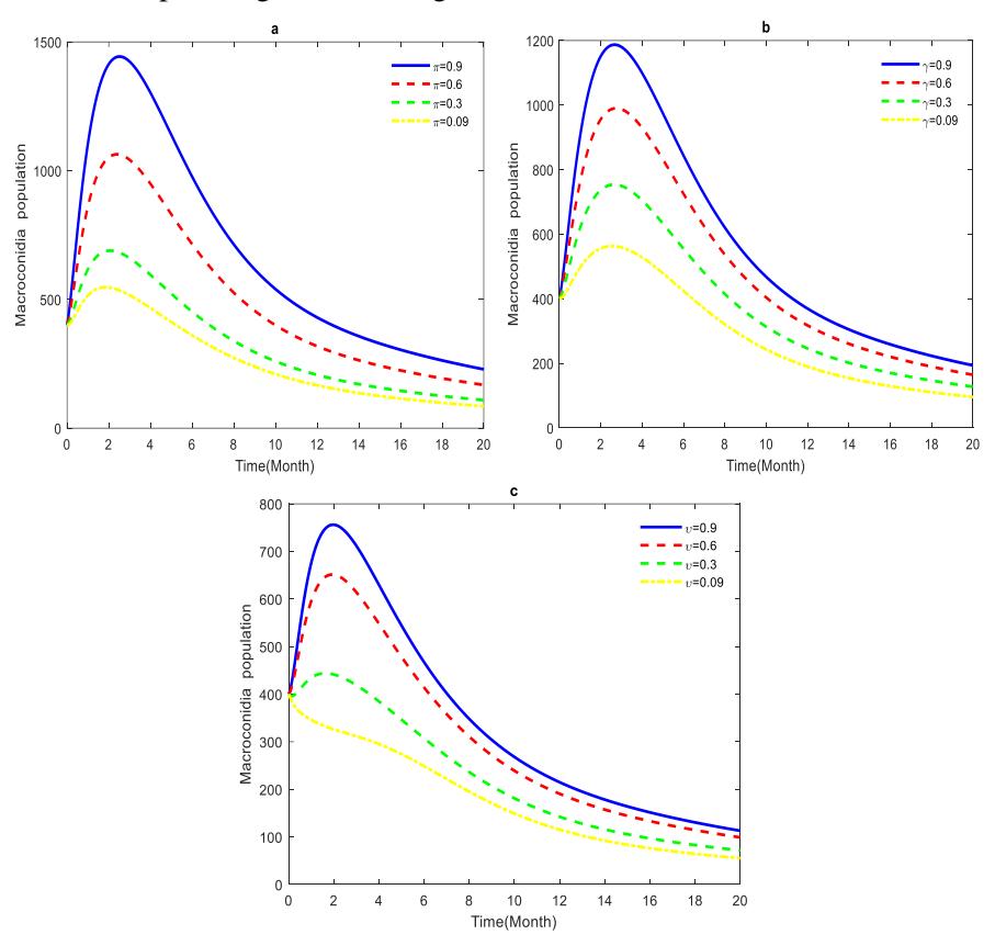
Figures 6 (a) Macroconidia spores population increases due to decomposition of diseased-induced dead plants. (b) Macroconidia spores population increases due to the decay of infected dead plants. (c) Macroconidia spores population increases due to the deterioration of exposed dead plants.
5.4 Effect of Decomposed Disease-Induced Dead Plants on Chlamydospores Growth
Figure 7 illustrates the impact of chlamydospore growth in the soil due to an increase of the amount of decomposed disease-induced plants. Decomposed disease-induced plants produce macroconidia spores. Macroconidia spores produce chlamydospores after the decomposition of dead plants since the environment is not conducive to the survival of macroconidia. Chlamydospores have thick walls, enabling them to survive in the dry season and increase disease transmission in a conducive environment. Chlamydospore saturation in the ground causes disease outbreak, which reduces the number of susceptible plants in the field. The number of susceptible plants decreases after the disease progresses to exposed plants. Initially, the number of exposed plants increases up to a certain level before reducing due to the transformation of infected plants. The macroconidia population decreases due to the production of chlamydospores.
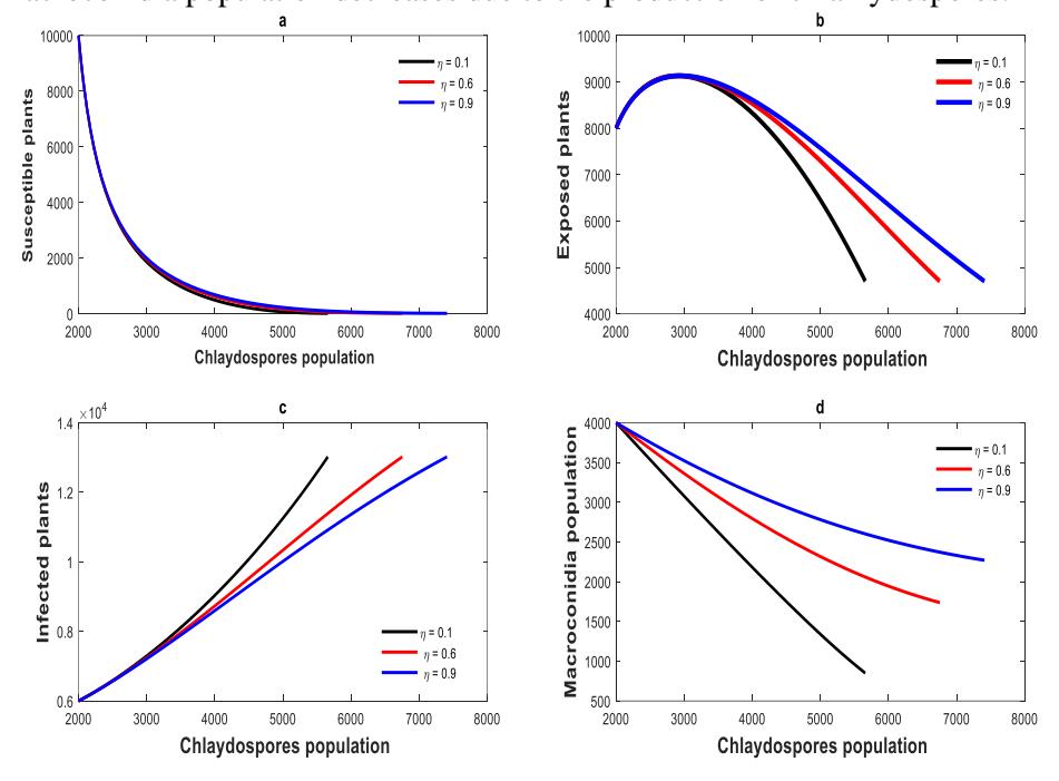
Figure 7 (a) Susceptible plant populations decline as more plants are exposed to the disease. (b) More plants become exposed because the interaction rate increases (c) An infected plants increase due to the rise of chlamydospores in the ground. (d) An increase in chlamydospores in the soil leads to a decrease in macroconidia spores.
6 Conclusion
This study addressed the role of decomposed disease-induced dead plants in the spread of cashew Fusarium wilt disease. Significant financial losses are caused by the disease, particularly for people or communities that depend on the cashew industry. Sensitivity analysis was conducted to consider the expected uncertainty in parameter values. It was discovered through local and global sensitivity analyses that various factors contribute to the disease's persistence and transmission. A critical factor during outbreaks are decayed disease-induced dead plants. The numerical solution determined the production of macroconidia from decayed disease-induced dead plants that contribute to the production of chlamydospores. The decomposition plays a vital role in ecosystems for nutrient redistribution in the soil. However, since it consists of disease-induced dead plants, this process increases chlamydospore saturation in the ground and hence disease prevalence and spread during an outbreak. Therefore, the presence of decomposed disease-induced dead plants should be considered when developing efficient methods of managing the infection rate during an outbreak.