
1 Introduction
The productivity quality in manufacturing or service companies should continuously be assessed and improved. The control chart has an important role in improving and maintaining the quality of the process. It is commonly used to examine and decide if the process state is statistically controlled or not. A process is considered to be in-control (IC), under normality distribution, as long as it has a constant mean and standard deviation. When there is a change in the
Received October 29<sup>th</sup>, 2021, Revised June 22<sup>th</sup>, 2023, Accepted for publication July 4<sup>th</sup>, 2023 Copyright © 2023 Published by ITB Institute for Research and Community Services, ISSN: 2337-5760, DOI: 10.5614/j.math.fund.sci.2023.55.1.4
process mean or standard deviation, the control chart triggers an alarm, indicating that the process is considered out-of-control (OC).
There are phenomena, for instance in chemical and biological assays, in which the mean and standard deviation vary over time, but those are naturally occurring IC processes. Although the respective mean and standard deviation control charts show the OC process, it is possible to consider the process as IC when its quotient is steady around a certain value [1]. This quotient is between the standard deviation σ relative to the mean µ, and is called the coefficient of variation (CV), γ. Process monitoring using CV is applicable in mechanical engineering [3], manufacturing [2], and materials engineering [4-6].
Kang et al. [7] introduced the first control chart for monitoring the coefficient of variation (CV), known as the SH-CV chart, which follows the Shewhart-type chart. Nevertheless, employing this chart to identify small to moderate shifts in CV is not advisable due to its limited sensitivity. Some further investigations have been conducted to strengthen the sensitivity of the SH-CV chart. The twosided EWMA-CV chart was developed by [8], while the one-sided EWMA-CV chart was elaborated in [9]. Both charts demonstrated a performance superior to the SH-CV chart in detecting small to moderate shifts in the coefficient of variation.
Furthermore, some researchers have proposed adaptive-type control chart implementation in order to improve OC detection, especially through variable sampling interval (VSI) and variable sample size (VSS) schemes. VSI and VSS methods of the Shewhart type for CV monitoring were proposed by Castagliola et al. in 2013 and 2015 [4,10], called VSI-CV and VSS-CV charts, respectively. Both charts have better performance compared to the SH-CV chart. Meanwhile the VSS-CV and VSI-CV charts were enhanced for short production runs ([11,12]). Further, a combination of VSS and VSI in observing the process can be executed by using the CV, which is called a VSSI-CV chart [13].
The VSI and VSS ideas were used in the Double Sampling (DS) chart. When an OC warning or signal occurs, the second sample is taken in the shortest time interval as an addition to the first sample. Croasdale [14] proposed the first DS chart for mean process monitoring (denoted as CDS-̅ chart). The information from both samples is evaluated independently by CDS-̅ chart. A modified CDS-̅ chart is executed by utilizing information from both samples in the second stage and is denoted as DS-̅ [15]. The DS procedure offers better statistical efficiency without increased sampling compared to the Shewhart chart. Alternatively, the procedure can reduce sampling without losing statistical efficiency. Irianto and Shinozaki [16] explored the effectiveness of both DS procedures and found that the DS chart proposed by Daudin outperformed the Croasdale chart regarding its ability to detect shifts.
Meanwhile, in terms of monitoring variability using the DS scheme, several authors, such as He & Grigoryan [17], developed the properties of the DS-s chart. Costa [18] proposed a DS scheme for improved the performance of the R chart and Lee & Khoo [19] investigated an economic-statistical design of the DS-s chart. The DS scheme for monitoring CV was proposed earlier by Ng et al. [20]. This chart outperforms the SH-CV chart in detecting small to moderate shifts in the CV. However, this chart procedure revealed that the condition of the second-stage process is based only on information from the second sample. On the other hand, Daudin [15] argued that more economies could be achieved by designing a scheme that involves information from the first sample in the second stage.
Therefore, the objectives of this study were: (a) to modify the procedure of the previous DS-CV chart, referred to as MDS-CV chart, by incorporating information from both samples when making decisions for the second stage; (b) to evaluate the performance of the MDS-CV chart and compare it with the DS-CV chart; and (c) to apply this chart to real data from a molding process as a case study. It should be noted that, alongside the preparation for this paper, similar research has been done that discussed another DS-CV chart that also considers information from both samples in making decisions for the secondstage process. However, that study used combined CV statistics as the weighted average of the first- and second-stage sample CVs. Meanwhile, the present paper used combined CV statistics as the total sample CV, calculated based on the ratio between the combined standard deviation and the combined mean of the first- and second-stage samples.
The rest of this paper is arranged as follows. In Section 2, the distribution of the sample CV is reviewed, including some notations used in this paper. The review of the DS-CV chart and the design of the modified chart and its statistical properties are explained in Section 3. An analysis of the numerical and a performance comparison with the DS-CV control chart is given in Section 4. An application example as a case study from a molding process is discussed in Section 5. In the last section, the conclusions are drawn.
2 Distribution of the Combined Sample CV
Suppose is a random variable and has positive values. It is taken from a population whose mean and standard deviation respectively are and , < ∞. Thus, the CV of , notated by , is expressed as:
\[\gamma = -\frac{\sigma}{\mu} \tag{1}\]
Assume that \(X_1, X_2, ..., X_n\) are random samples with size n and follows a normal distribution \(N(\mu, \sigma^2)\). Let the sample mean \((\bar{X})\) and standard deviation (S) of samples be calculated as follows, respectively:
\[\bar{X} = \frac{1}{n} \sum_{i=1}^{n} X_i; \quad S = \left(\frac{\sum_{i=1}^{n} (X_i - \bar{X})^2}{n-1}\right)^{1/2}\] (2)
The sample CV, symbolized by G, is defined as:
\[G = \frac{S}{\overline{X}} \tag{3}\]
For \(0 < \gamma \le 0.5\), the non-central t distribution can accurately approximate the cumulative distribution function (CDF) of G [21]. The CDF of G approximation is:
\[F_G(x|n,\gamma) = 1 - F_T(\sqrt{n}/x|n-1,\sqrt{n}/\gamma), \qquad x > 0\] (4)
where \(F_T(.)\) is the CDF of the non-central t distribution with degree of freedom is n-1 and the parameter of non-centrality is \(\sqrt{n}/\gamma\). The inverse CDF of G, \(F_G^{-1}(\alpha|n,\gamma)\) is obtained by inverting \(F_G(x|n,\gamma)\) as follows:
\[F_G^{-1}(\alpha|n,\gamma) = \frac{\sqrt{n}}{F_T^{-1}(1-\alpha|n-1,\sqrt{n}/\gamma)}\] (5)
where \(F_T^{-1}(.)\) is the inverse CDF of the noncentral t distribution.
Furthermore, because this study modified the DS chart for monitoring the CV, based on the concept that if the statistic from the first sample fall into the warning area, it needs to be confirmed using information from the second sample. This is carried out by calculating the combined statistics from the first and the second sample in order to make a decision on the process state. Since the statistic to be monitored is CV, then the properties of the combined sample CV in the second stage are needed.
Suppose that \(X_1 = \{X_{11}, X_{12}, ..., X_{1n_1}\}\) and \(X_2 = \{X_{11}, X_{12}, ..., X_{1n_2}\}\) are random sample collections from a normal \(N(\mu, \sigma^2)\) distribution of size \(n_1\) and \(n_2\), respectively. Let \(\bar{X}_k\) and \(S_k\) be the \(k^{\text{th}}\) sample mean and standard deviation of \(X_k\), with k = 1, 2, calculated by Eq. (2). Let the combined sample mean \((\bar{X}_c)\) and sample standard deviation \((S_c)\) be defined as follows, respectively:
\[\bar{X}_c = \frac{n_1 \cdot \bar{X}_1 + n_2 \cdot \bar{X}_2}{n_1 + n_2}\] and \(S_c = \left(\frac{(n_1 - 1)S_1^2 + (n_2 - 1)S_2^2}{n_1 + n_2 - 2}\right)^{1/2}\), (6)
then the combined sample CV is defined as [22]:
\[G_c = \frac{S_c}{\bar{X}_c},\tag{7}\]
Further, to investigate the distribution of \(G_c\), first we propose the following lemma.
<u>Lemma.</u> The distribution of \(T = (\sqrt{n_1 + n_2})\bar{X}_c/S_c\) follows a non-central t distribution with degree of freedom \(v = (n_1 + n_2 - 2)\) and non-centrality parameter \(\delta = \sqrt{n_1 + n_2}\), \(\mu/\sigma\).
Proof:
Consider that \(\bar{X}_k \sim N(\mu, \sigma^2/n_k)\) and \(\frac{(n_k-1)S_k^2}{\sigma^2} \sim \chi^2_{(n_k-1)}\), for k=1,2. Then,
\[\bar{X}_c \sim N(\mu, \sigma^2/(n_1 + n_2))\] and \(\frac{n_1 + n_2 - 2)S_k^2}{\sigma^2} \sim \chi^2_{(n_1 + n_2 - 2)}\).
Notice that \(\bar{X}_k\) is independent of \(S_k^2\) for k=1,2. Since \(\bar{X}_c\) is a function of \(\{\bar{X}_1,\bar{X}_2\}\) and \(S_c^2\) is a function of \(\{S_1^2,S_2^2\}\), \(\bar{X}_c\) is independent of \(S_c^2\). Note that
\[\begin{split} \frac{\sqrt{n_1 + n_2} \bar{X}_p}{S_p} &= \frac{\sqrt{n_1 + n_2} (\bar{X}_p - \mu) + \sqrt{n_1 + n_2} \mu}{\sqrt{S_p^2}} \\ &= \frac{\frac{(\sqrt{n_1 + n_2}) (\bar{X}_p - \mu)}{\sigma} + \frac{(\sqrt{n_1 + n_2}) \mu}{\sigma}}{\sqrt{\frac{(n_1 + n_2 - 2)S_p^2}{(n_1 + n_2 - 2)\sigma^2}}} \\ &= \frac{Z + (\sqrt{n_1 + n_2}) \mu / \sigma}{\sqrt{W / (n_1 + n_2 - 2)}} = \frac{Z + \delta}{\sqrt{W / \nu}} = T \end{split}\]
Since \(Z \sim N(0,1)\) and \(W \sim \chi^2_{n_1+n_2-2}\), T follows a non-central t distribution with degree of freedom \(v = (n_1 + n_2 - 2)\) and non-centrality parameter \(\delta = (\sqrt{n_1 + n_2})\mu/\sigma\).
Based on the lemma above, the CDF of \(G_c\) is determined as stated in the following corollary:
Corollary. The CDF of \(G_c\) is given as follows:
\[F_{G_c}(x|n_1+n_2,\gamma) = 1 - F_t\left(\frac{\sqrt{n_1+n_2}}{x}\left|n_1+n_2-2,\frac{\sqrt{n_1+n_2}}{\gamma}\right.\right) \tag{8}\] where \(F_t(.|\nu,\delta)\) is a non-central t distribution with parameter of non-centrality \(\delta = (\sqrt{n_1 + n_2})/\gamma\) and degree of freedom \(\nu = (n_1 + n_2 - 2)\).
Proof
\(\overline{Since} G_c = \frac{S_c}{\bar{X}_c}\) it means that:
\[\begin{split} F_{G_c}(x|n_1+n_2,\gamma) &= P(G_c \leq x) = P\left(\frac{\sqrt{n_1+n_2}}{G_c} \geq \frac{\sqrt{n_1+n_2}}{x}\right) \\ &= P\left(\frac{\sqrt{n_1+n_2}.\bar{X}_c}{S_c} \geq \frac{\sqrt{n_1+n_2}}{x}\right) \\ &= P\left(T \geq \frac{\sqrt{n_1+n_2}}{x}\right) = 1 - P\left(T \leq \frac{\sqrt{n_1+n_2}}{x}\right). \end{split}\]
Using Lemma 1, the CDF of \(G_c\) is obtained as follows:
\[F_{G_c}(x|n_1+n_2,\gamma) = 1 - F_t\left(\frac{\sqrt{n_1+n_2}}{x}\left|n_1+n_2-2,\frac{\sqrt{n_1+n_2}}{\gamma}\right|\right)\]
3 Modified Double Sampling Coefficient of Variation Chart
Suppose that \(X_{1t}, X_{2t}, ..., X_{nt}\) are random samples of size n whose distributions are normal \(N(\mu_t, \sigma_t^2)\) and \(\mu_t\) and \(\sigma_t^2\) respectively are the mean and variance of the population at number of observations t=1, 2, .... Define the CV when the IC process is \(\gamma_t = \sigma_t/\mu_t = \gamma_0\). Thus, the CV, \(\gamma_t = \sigma_t/\mu_t\) must be identical with fixed IC value \(\gamma_0\) for all number of observations, t, although the values of \(\mu_t\) and \(\sigma_t\) may be different between one subgroup and another.
3.1 A Brief Review of DS-CV Chart
Here, the DS-CV chart proposed by Ng et al. [20] is briefly reviewed. A schematic view of the DS-CV chart is shown in Figure 1, where the lower/upper warning limits (LWL/UWL) of this chart in Stage 1 are defined as:
\[LWL = \mu_0(G) - W\sigma_0(G)\]; \(UWL = \mu_0(G) + W\sigma_0(G)\)
and the lower/upper control limits \((LCL_k/UCL_k)\) in Stage k, k=1,2, are defined as:
\[LCL_k = \mu_0(G) - L_k \sigma_0(G); \ UCL_k = \mu_0(G) + L_k \sigma_0(G)\] where W > 0 is the warning limit and \(L_1 > W\) is the control limit for the parameters of the first stage, and \(L_2 > 0\) is the control limit for the parameters of the second stage.
For the sample CV, G, the IC-mean and IC-standard deviation are represented by \(\mu_0(G)\) and \(\sigma_0(G)\) respectively. The formulas \(\mu_0(G)\) and \(\sigma_0(G)\) can be found from the work of Castagliola [4]. Let
\[I_1 = [LWL, UWL], \quad I_2 = [LCL_1, LWL), \quad I_3 = (UWL, UCL_1],\] and \[I_4 = (UCL_1, +\infty) \cup (-\infty, LCL_1).\] \[UCL_1 - \frac{\text{Out-of-control } (I_4)}{\text{Take a second sample } (I_2)}\] \[UCL_2 - \frac{\text{In-control } (I_1)}{\text{LUL}}\] \[LCL_1 - \frac{\text{Take a second sample } (I_3)}{\text{Out-of-control } (I_4)}\] \[ECL_2 - \frac{\text{Second Stage}}{\text{Second Stage}}\]
Figure 1 Schematic view of the DS-CV chart. An out-of-control signal is detected under three conditions, namely if (i) the first-stage sample falls at \(I_4\), (ii) the first-stage sample falls at \(I_2\) and the second-stage sample falls above \(UCL_2\), or (iii) the first-stage sample falls at \(I_3\), and the second-stage samples fall below \(LCL_2\).
Based on Figure 1, the DS-CV chart procedure as follows [17]:
- Step 1. Observe the 1<sup>st</sup> sample with size \(n_1\) at sample number t, i.e., \(X_{1it}\), \(i = 1,2,...,n_1\) from a normally distributed population with mean \(\mu_t\) and standard deviation \(\sigma_t\).
- Step 2. Determine the 1<sup>st</sup> sample CV, \(G_{1t} = S_{1t}/\bar{X}_{1t}\), where \(\bar{X}_{1t}\) and \(S_{1t}\) are the 1<sup>st</sup> sample mean and the standard deviation, respectively.
- Step 3. If \(G_{1t} \in I_1\), then the IC process is declared and returns to Step 1 for time (t+1).
- Step 4. If \(G_{1t} \in I_4\), then continue to Step 7.
- Step 5. If \(G_{1t} \in I_2 \cup I_3\), observe the \(2^{\text{nd}}\) sample with size \(n_2\), i.e., \(X_{2it}\), \(i = 1,2,\ldots,n_2\) from the \(1^{\text{st}}\) sample population. Do the evaluation to the \(2^{\text{nd}}\) sample CV, \(G_{2t} = S_{2t}/\bar{X}_{2t}\), where \(\bar{X}_{2t}\) and \(S_{2t}\) are the \(2^{\text{nd}}\) sample mean and standard deviation, respectively.
- Step 6. If \((G_{1t} \in I_2 \text{ and } G_{2t} \ge LCL_2)\) or \((G_{1t} \in I_3 \text{ and } G_{2t} \le UCL_2)\), the IC process is declared, then returns to Step 1 for sample number (t+1). Otherwise, continue to Step 7.
- Step 7. The OC signal is detected by the DS-CV chart at \(t^{th}\) sample. Immediate actions are required to distinguish the assignable causes(s).
Suppose that an IC process given a process CV, , that takes into account information from both samples using the DS scheme, has probability (), which is defined as:
\[P_a(\gamma) = P_{a1}(\gamma) + P_{a2}(\gamma), \tag{9}\] where 1() and 2() are the probabilities of the declared IC process in the first and the second stage, given a process CV, respectively. According to the above procedure, Ng et al. [18] derived the probabilities formula as:
\[\begin{split} P_{a1}(\gamma) &= Pr(LWL \leq G_{1t} \leq UWL) = F_G(UWL|n_1, \gamma) - F_G(LWL|n_1, \gamma) \\ P_{a2}(\gamma) &= Pr(LCL_1 \leq G_{1t} \leq LWL \text{ and } G_{2t} \geq LCL_2) \\ &+ Pr(UWL \leq G_{1t} \leq UCL_1 \text{ and } G_{2t} \leq UCL_2) \\ &= \{ [F_G(LWL|n_1, \gamma) - F_G(LCL_1|n_1, \gamma)] \times [1 - F_G(LCL_2|n_2, \gamma)] \} + \\ &\{ [F_G(UCL_1|n_1, \gamma) - F_G(UWL|n_1, \gamma)] \times F_G(LCL_2|n_2, \gamma) \} \end{split}\] where (|, ) is expressed in Eq. (4).
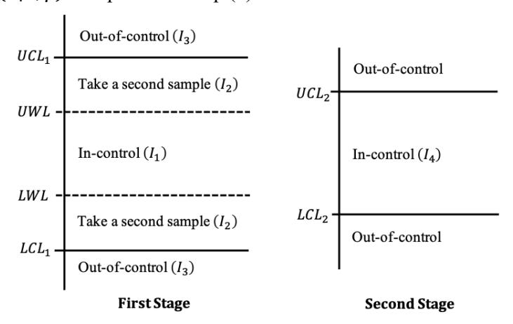
Figure 2 Schematic view of the MDS-CV chart. An out-of-control signal is detected under two conditions, i.e., if (i) the first-stage sample falls at 3 , (ii) the first-stage sample falls at 2 and the second-stage sample falls above 2 or below 2 .
Based on the DS-CV chart procedure, it can be seen that the determination of the process conditions in Stage 2 is only judged by the CV of the second sample. In contrast, the DS idea should use the information combination from the first and second samples for examining the process condition in Stage 2 ([15,17]). Thus, a modification of the DS-CV chart is suggested. This modification involves information from the first and the second sample in order to obtain the conclusion for the second stage.
3.2 Proposed Chart
In this section, the modified DS chart for monitoring the CV, denoted by MDS-CV chart, is described. Redefine the intervals of Figure 1 to obtain the modified chart, where \(I_1 = (LCL_1, UCL_1]\) \(I_2 = [LCL_1, LWL) \cup (UWL, UCL_1]\), \(I_3 = (-\infty, LCL_1) \cup (UCL_1, +\infty)\), and \(I_4 = (LCL_2, UCL_2]\), which is illustrated in Figure 2. The operational procedure for this chart is:
Run the DS-CV chart procedure, by modifying Step 4 to 6, as follows:
Step 4. If \(G_{1t} \in I_3\), then continue to Step 7.
- Step 5a. If \(G_{1t} \in I_2\), observe the \(2^{\rm nd}\) sample of size \(n_2\), \(X_{2it}\), \(i=1,2,\ldots,n_2\) from the \(1^{\rm st}\) sample population. Calculate \(\bar{X}_{2t}\) and \(S_{2t}\) as the \(2^{\rm nd}\) sample mean and standard deviation, respectively.
- Step 5b. Evaluate the combined sample CV, \(G_{ct} = S_{ct}/\bar{X}_{ct}\), where \(\bar{X}_{ct}\) and \(S_{ct}\) are the combined sample mean and standard deviation, which are computed using Eq. (7).
- Step 6. If \(G_{1t} \in I_2\) and \(G_{ct} \in I_4\), the IC process is declared, and return to Step 1 for sample number (t + 1). Else, continue to Step 7.
Furthermore, the properties of the MDS-CV chart were investigated. Let \(P_a(\gamma)\) in Eq. (9) for our chart is denoted as \(P_a^*(\gamma)\), then this probability is defined as:
\[P_{a}^{*}(\gamma) = P_{a1}^{*}(\gamma) + P_{a2}^{*}(\gamma). \tag{10}\]
According to this chart procedure, the probabilities \(P_{a1}^{*}(\gamma)\) and \(P_{a2}^{*}(\gamma)\) are derived as follows:
\[\begin{split} P_{a1}^{*}(\gamma) &= P_{a_{1}}(\gamma) \\ P_{a2}^{*}(\gamma) &= Pr\{(LCL_{1} \leq G_{1t} \leq LWL \text{ or } UWL \leq G_{1t} \leq UCL_{1}) \text{ and } (LCL_{2} \\ &\leq G_{ct} \leq UCL_{2})\} \\ &= P_{2}(\gamma). \left[ F_{G_{c}}(UCL_{2}|n_{1} + n_{2}, \gamma) - F_{G_{c}}(LCL_{2}|n_{1} + n_{2}, \gamma) \right] \end{split}\] and
\[P_{2}(\gamma) = [F_{G}(UCL_{1}|n_{1},\gamma) - F_{G}(UWL|n_{1},\gamma)] + [F_{G}(LWL|n_{1},\gamma) - F_{G}(LCL_{1}|n_{1},\gamma)]\] (11)
is the probability that the 1<sup>st</sup> sample CV falls inside the warning area. \(F_G(.|n_1,\gamma)\) is calculated using Eq. (4), while \(F_{G_c}(.|n_1+n_2,\gamma)\) is calculated using Eq. (8).
Furthermore, to evaluate this chart, the average sample size (ASS) and the average run length (ARL) are implemented. Based on the DS scheme, ARL is defined as:
\[ARL = \frac{1}{1 - P_a^*(\gamma)} \tag{12}\] while ASS at each observation is calculated as:
\[ASS = n_1 + n_2 P_2(\gamma) \tag{13}\] where \(P_a^*(\gamma)\) and \(P_2(\gamma)\) are calculated using Eq. (10) and Eq. (11).
If the CV of the IC-process is represented by \(\gamma = \gamma_0\), then the CV of the OC-process arises while \(\gamma = \gamma_1\), i.e., \(\gamma_1 = \tau \gamma_0\) for a specific shift \(\tau \neq 1\), where \(\tau\) is the CV shift size. The upward and downward shifts in CV are denoted as \(\tau > 1\) and \(\tau \in (0,1)\), respectively. The IC (OC) ARL is denoted as \(ARL_0\) (\(ARL_1\)), while the IC (OC) ASS is denoted as \(ASS_0\) (\(ASS_1\)). Using Eq. (12) and Eq. (13), the warning and control limits of this chart are determined such that:
\[ARL_0 = ARL(\tau = 1) = \frac{1}{1 - P_a^*(\gamma_0)} = \frac{1}{\alpha_0}\] where \(\alpha_0\) is the probability of a false alarm (error type-I) and
\[ASS_0 = ASS(\tau = 1) = n_1 + n_2 P_2(\gamma_0)\]
4 Performance Evaluation and Comparison
4.1 Performance Evaluation of the MDS-CV Chart
The performance of the MDS-CV chart is assessed based on the ARL criteria. The optimization model is defined as follows:
\[\min_{W, L_1, L_2} ARL_1 = \min_{W, L_1, L_2} \frac{1}{1 - P_a^*(\gamma_1)}\] (14)
Subject to:
- (a) \(ASS_0 = n_0\), where \(n_0\) is the desired in-control ASS
- (b) \(ARL_0 = \ell\), where \(\ell\) is the desired in-control ARL
- (c) \(2 \le n_1 < n_0 < n_1 + n_2 \le n_{max}\)
The steps of finding the optimal parameter \((W, L_1, L_2)\) of MDS-CV charts are:
- 1. Choose the desired \(\gamma_0\), \(n_0\), \(\ell\), and \(\tau\) values.
- 2. For the IC condition \((\tau = 1)\), choose \(n_1\) and \(n_2\) variations that satisfy constraint (c); all possible values of W and \(L_1\) are obtained from constraint (a).
- 3. For all fixed values of W and \(L_1\) found in Step 2, all values of \(L_2\) can be obtained from constraint (b).
- 4. For any out-of-control condition (\(\tau \neq 1\)), find the optimal parameter that minimizes Eq. (14) from all possible combinations of triple parameters found in Steps 2 and 3.
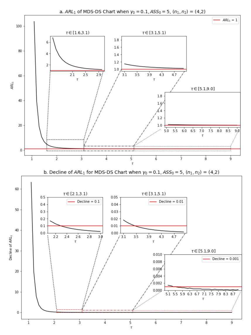
Figure 3 (a) Performance of the MDS-CV chart and (b) decrease of \(ARL_1\), based on \(ARL_1\) value, when \(\gamma_0 = 0.1\), \(ARL_0 = 370.4\), \(ASS_0 = 5\), and \((n_1, n_2) = (4,2)\) for \(\tau = [1.1,9.0]\). The \(ARL_1\) value decreased as the \(\tau\) value increased, meaning that when the shift increased, the MDS-CV chart will be faster in detecting out-of-control signals. In the range \(1 < \tau \le 2\), the decline is almost 97 times faster than the decline in the range \(2 \le \tau < 3.1\).
Based on the optimization model above, the performance of MDS-CV chart can be evaluated in two ways. First, the effect of \(\tau\) when \(n_1\) and \(n_2\) are fixed. Here the performance of MDS-CV chart was investigated for \(\gamma_0 = 0.1\), \(ARL_0 = 0.1\)
370.4, \(ASS_0 = 5\), and \((n_1, n_2) = (4,2)\), for \(\tau = [1.1,9.0]\), as provided in Figure 3.
Figure 3(a) shows that the \(ARL_1\) value decreased as the value of \(\tau\) increased, with a swift decline in the range \(1 < \tau \le 2\), i.e., almost 97 times faster than the decrease in the range \(2 \le \tau < 3.1\), and gets slower when \(\tau \ge 3.2\), until it converges to a value of 1. More specifically, Figure 3(b) shows a decrease of \(ARL_1\) less than 0.1 when \(\tau > 2.3\), and less than 0.01 when \(\tau > 3.5\). This means that when the shift size of the CV increases, the MDS-CV chart will exhibit faster detection of such shifts.
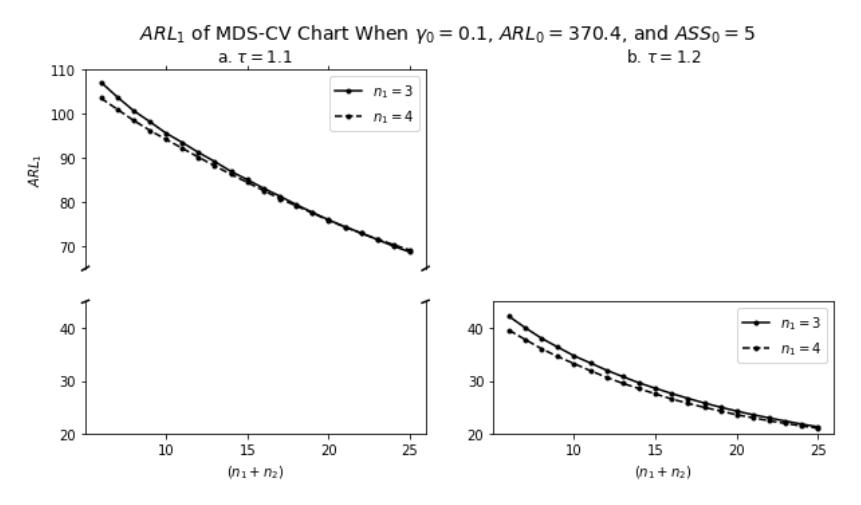
Figure 4 Performance of the MDS-CV chart based on the \(ARL_1\) value, when \(\gamma_0 = 0.1\), \(ARL_0 = 370.4\), \(ASS_0 = 5\), for \(n_1 = \{3,4\}\) and variation of \(n_{tot} = n_1 + n_2 = \{6,7,...,25\}\) with \(\tau = 1.1\) (left) and \(\tau = 1.2\) (right).
The second way, investigate the effect of \(n_1\) and \(n_2\) when \(\tau\) is fixed. The performance of MDS-CV chart when \(\gamma_0=0.1\), \(ARL_0=370.4\), \(ASS_0=5\), and \(\tau=\{1.1,1.2\}\), for \(n_1=\{3,4\}\) and variation of \(n_{tot}=n_1+n_2=\{6,7,\dots,25\}\) can be seen in Figure 4.
Based on Figure 4, when \(\tau\) is fixed, the \(ARL_1\) value decreased as \(n_{tot}\) increased, either \(n_1=3\) or \(n_1=4\). This means that when the sample size is increased, the sensitivity of the MDS-CV chart improves in detecting out-of-control signals. Moreover, generally, the value of \(ARL_1\) for \(n_1=4\) is smaller than the value of \(ARL_1\) for \(n_1=3\), but when \(\tau=1.1\) and \(n_{tot}\geq 23\), the \(ARL_1\) value reserved for \(n_1=3\) is smaller. This indicates that the selection of the first sample size has an influence on the performance of the chart.
4.2 Comparison with the DS-CV Chart
A comparison of our modified chart with the DS-CV chart was done based on \(ARL_1\) terms. A control chart is deemed superior to its competitors if it possesses a smaller \(ARL_1\) value when the \(ARL_0\), \(ASS_0\), and \(\tau\) values are fixed. In this paper, the comparisons discussed are limited to values \(\gamma_0 = 0.1\), \(ARL_0 = 370.4\), \(ASS_0 = 5\), and \(\tau = \{1.1,1.2\}\), for \(n_1 = \{3,4\}\) and variation of \(n_{tot} = n_1 + n_2 = \{6,7,...,25\}\). The \(ARL_1\) comparison of both charts can be seen in Figure 5.
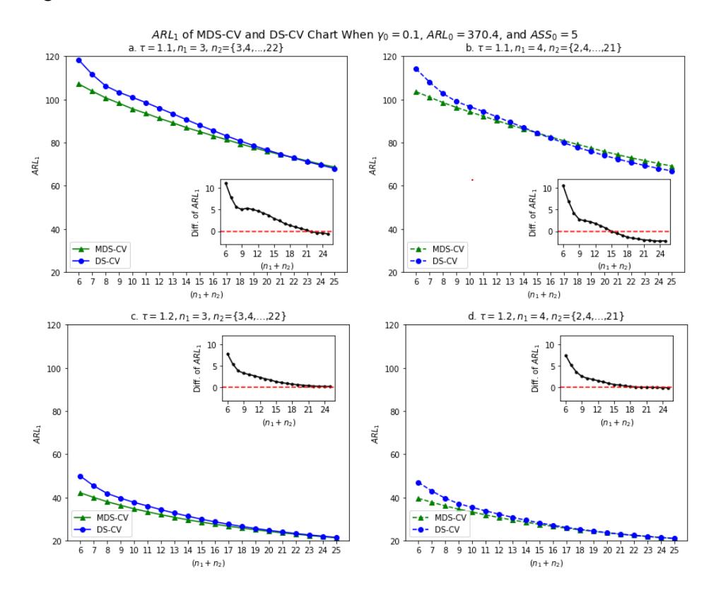
Figure 5 Performance comparison between the MDS-CV and DS-CV charts based on \(ARL_1\) when \(\gamma_0 = 0.1\), \(ARL_0 = 370.4\), and \(ASS_0 = 5\), for (a). \(\tau = 1.1\), \(n_1 = 3\); (b). \(\tau = 1.1\), \(n_1 = 4\); (c). \(\tau = 1.2\), \(n_1 = 3\); and (d). \(\tau = 1.2\), \(n_1 = 4\). Inside the charts are different values of \(ARL_1\), where Diff. of \(ARL_1 = ARL_{1(DS-CV)} - ARL_{1(MDS-CV)}\).
Figure 5 shows that for \(\tau = 1.1\) and 1.2, the \(ARL_1\) value of the MDS-CV chart \((ARL_{1-MDS})\) is smaller than the \(ARL_1\) value of the DS-CV chart \((ARL_{1-DS})\). However, with increasing size of \(n_{tot}\), the difference between \(ARL_{1-MDS}\) and \(ARL_{1-DS}\) is getting smaller, and for a certain \(n_{tot}\), the \(ARL_{1-DS}\) reverses to smaller than 1−. For instance, for = 1.1 1 = 3, < 22, 1− is smaller than 1−, but since ≥ 22, 1− is smaller than 1−. This means that the performance of the MDS-CV chart surpasses that of the DS-CV chart, especially when the total number of samples ≤ 15. However, for a larger , the MDS-CV chart's performance was almost equal to that of the DS-CV chart and even the DS-CV's performance was better than that of the MDS-CV chart.
5 Application Illustration: A Case Study
This section presents a practical demonstration of the DS-CV chart by applying it to a real industrial company. The case study focused on evaluating the quality of the steel molding process at heavy equipment companies located in DKI Jakarta, Indonesia. The quality characteristics of concern were the result of measuring the chemical composition of the type of material (consisting of carbon, silicon, manganese, phosphor, nickel, chrome, and others) used for steel molding. At each time of inspection (observation), the chemical composition was measured on the same type of material. The type of material can change at every inspection depending on the type of material scheduled to be produced. Therefore, in the IC process state, the mean chemical composition can change from one observation to another.
In this study, the chemical composition to be processed is carbon (C) in units of percentage by weight, because this substance is a key factor in the quality of steel molding, which affects the level of hardness and the tensile strength. The data obtained were secondary data from manual check sheet records of monthly chemical composition measurements for three types of materials, namely type 2H, type 1H, and type 3E, from January 2017 to December 2018. In terms of carbon composition, the materials had the following specifications: type 2H (0.40-0.47), type 1H (0.28-0.35), and type 3E (0.27-0.30). The interest in this case study was to monitor the quality of the steel molding process based on the variability of the carbon composition.
In order to apply the proposed chart in controlling the variability of the carbon composition, some assumptions had to be met. Those were: (1) the sample for each observation is normally distributed; (2) the samples between observations are independent of each other; and (3) the mean and standard deviation between observations can change but have a proportional relationship against the CV. Therefore, in this case, more than one type of material must be involved to fulfill the third assumption. The randomness of the material type order, which is the sample in this study, is unnecessary. This is because the material type order depends on the number of requests for heavy equipment products that require
steel molds from each type of material. The analysis of randomness is not discussed in this study and is a problem limitation.
Table 1 Statistics from the Phase I data set (carbon composition of the material in 2017), consisting of 26 observations (unit sample is per two weeks) and three types of material (2H, 1H* , and 3E**) with sample size 0 = 5. The data set was used to estimate the in-control CV process, 0 .
| Obs. | (𝑋̅ , 𝑆) | 𝐺𝑖 | Obs. | (𝑋̅ , 𝑆) | 𝐺𝑖 |
|---|---|---|---|---|---|
| 1 | (0.430 , 0.0100) | 0.0233 | 14* | (0.328 , 0.0084) | 0.0255 |
| 2 | (0.428 , 0.0192) | 0.0449 | 15* | (0.450 , 0.0122) | 0.0272 |
| 3 | (0.438 , 0.0130) | 0.0298 | 16* | (0.335 , 0.0112) | 0.0334 |
| * 4 | (0.332 , 0.0084) | 0.0252 | 17 | (0.428 , 0.0110) | 0.0256 |
| * 5 | (0.314 , 0.0114) | 0.0363 | 18* | (0.330 , 0.0158) | 0.0479 |
| 6 | (0.436 , 0.0089) | 0.0205 | 19** | (0.286 , 0.0055) | 0.0192 |
| 7 | (0.434 , 0.0207) | 0.0478 | 20** | (0.289 , 0.0042) | 0.0145 |
| 8 | (0.448 , 0.0130) | 0.0291 | 21** | (0.291 , 0.0074) | 0.0255 |
| 9 | (0.424 , 0.0114) | 0.0269 | 22* | (0.323 , 0.0084) | 0.0259 |
| 10** | (0.292 , 0.0045) | 0.0153 | 23* | (0.329 , 0.0124) | 0.0378 |
| 11 | (0.430 , 0.0100) | 0.0233 | 24 | (0.418 , 0.0096) | 0.0229 |
| 12 | (0.434 , 0.0152) | 0.0349 | 25* | (0.328 , 0.0084) | 0.0255 |
| 13* | (0.332 , 0.0130) | 0.0393 | 26** | (0.278 , 0.0057) | 0.0205 |
The data from 2017 used to determine the parameters of the process in an IC state was the Phase I data set (Start-up Stage Phase). While the data from 2018 used was the Phase II data set (Control Phase). The materials consisted of 46.2% observations from 2H, 34.6% observations from 1H, and 19.2% observations from 3E. Table 1 presents statistics of the data set, including the mean, standard deviation, and coefficient of variation of each observation.
Based on Table 1, it can be seen that 50% of the initial observations were dominated by the 2H material, while the remaining observations were quite evenly distributed. It shows that in the middle of the first year, the demand for steel molds of 2H was higher than for the other types of material. Afterward, based on Table 1, the process target and variability were monitored by the ̅ and S chart, as presented in Figure 6(a)-(b), while Figure 6(c) shows the linear regression of S to ̅ in Phase I. The test results showed that there is a constant proportional relationship, = × . This indicates that it is necessary to monitor the variability through a CV chart.
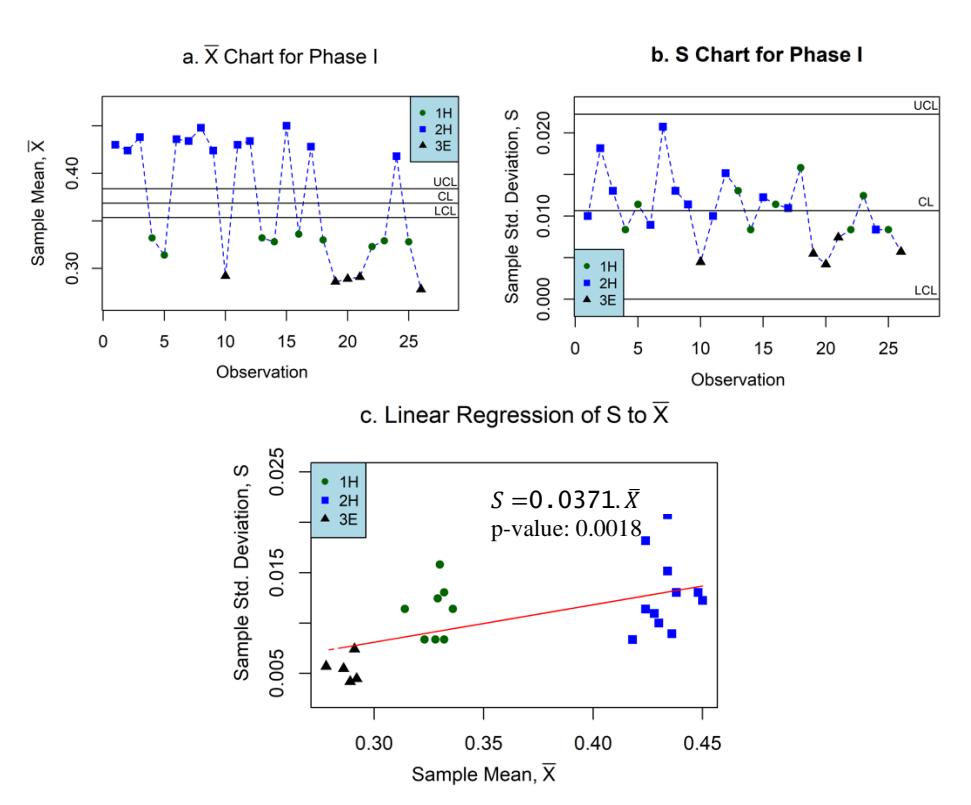
Figure 6 Process control based on (a) ̅-chart and (b) -chart, for the Phase I data set. Based on the mean, the process is OC, but the process is IC according to the S-chart. (c). Linear regression of S to ̅ in Phase I.
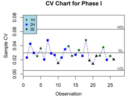
Figure 7 The CV chart for Phase I data set with = 5. Based on the CV, the process control is IC. This result was used to estimate the IC parameter of the CV process, 0 .
Figure 7 presents the CV chart for the Phase I data set. It can be seen that the process variability of the Phase I data set based on the CV is in the IC state.
Then, the IC parameter of the CV, \(\gamma_0\), could be estimated using the root-meansquare of \(G_i\), \(i=1,2,\ldots,m\), which was \(\bar{G}=0.030\), which was used as reference in determining the control limits in the process monitoring of the Phase II data set based on the DS-CV and MDS-CV charts.
Table 2 Phase II data set (carbon composition of material in 2018), consisting of 25 observations (unit sample is per two weeks) and three types of materials (2H, 1H*, and 3E**) with \(ASS_0 = 5\) and samples size \(n_1 = 3\), \(n_2 = 3\).
| Ol | E: St | Einst Store | Second Stage | ||||
|---|---|---|---|---|---|---|---|
| Obs. | First Stage | DS-CV Chart | MDS-CV Chart | ||||
| \((\bar{X}_1, S_1)\) | \(G_1\) | \((\overline{X}_2, S_2)\) | \(G_2\) | \((\bar{X}_c, S_c)\) | \(G_c\) | ||
| 1 | (0.443, 0.015) | 0.034 | |||||
| 2 3** | (0.420, 0.010) | 0.024 | No ne | ed to take | the second sample | ||
| 3** | (0.280, 0.009) | 0.031 | |||||
| 4** | (0.285, 0.005) | 0.018 | (0.278, 0.008) | 0.027 | (0.282, 0.006) | 0.023 | |
| 5** | (0.288, 0.006) | 0.020 | (0.287, 0.003) | 0.010 | (0.288, 0.005) | 0.016 | |
| 6 | (0.423, 0.015) | 0.036 | (0.430, 0.017) | 0.040 | (0.427, 0.016) | 0.038 | |
| 7** | (0.293, 0.008) | 0.026 | No ne | ed to take | the second sample | ||
| \(8^*\) | (0.313, 0.012) | 0.037 | (0.322, 0.010) | 0.032 | (0.318, 0.011) | 0.035 | |
| 9** | (0.287, 0.003) | 0.010 | (0.285, 0.005) | 0.018 | (0.286, 0.004) | 0.014 | |
| \(10^{*}\) | (0.319, 0.004) | 0.011 | (0.322, 0.003) | 0.009 | (0.320, 0.003) | 0.010 | |
| 11** | (0.285, 0.009) | 0.030 | |||||
| 12* | (0.320, 0.010) | 0.031 | No ne | ed to take | the second sample | ||
| 13* | (0.310, 0.009) | 0.028 | |||||
| 14 | (0.428, 0.019) | 0.044 | (0.427, 0.015) | 0.036 | (0.428, 0.017) | 0.040 | |
| 15* | (0.303, 0.020) | 0.067 | (0.312, 0.018) | 0.056 | (0.308, 0.019) | 0.062 | |
| 16* | (0.322, 0.016) | 0.050 | (0.318, 0.013) | 0.040 | (0.320, 0.014) | 0.045 | |
| \(17^{*}\) | (0.328, 0.010) | 0.032 | No ne | ed to take | the second sample | ||
| \(18^{*}\) | (0.320, 0.013) | 0.041 | (0.320, 0.010) | 0.031 | (0.320, 0.012) | 0.037 | |
| \(19^{*}\) | (0.320, 0.010) | 0.031 | No no | ad to take | the second sample | ||
| 20 | (0.427, 0.012) | 0.027 | ivo ne | ей ю шке | ine secona sampie | ||
| 21 | (0.413, 0.015) | 0.037 | (0.420, 0.010) | 0.024 | (0.417, 0.013) | 0.031 | |
| 22 | (0.428, 0.010) | 0.024 | No ne | ed to take | the second sample | ||
| 23 | (0.418, 0.024) | 0.056 | (0.415, 0.018) | 0.043 | (0.417, 0.021) | 0.050 | |
| \(24^{*}\) | (0.317, 0.013) | 0.040 | (0.312, 0.010) | 0.033 | (0.314, 0.012) | 0.037 | |
| 25* | (0.320, 0.010) | 0.031 | No ne | ed to take | the second sample | ||
Note: Based on the MDS-CV chart, there was an OC signal detected at the 15<sup>th</sup> observation (bold).
The Phase II data set (carbon composition data in 2018) consisted of 26 observations, with a total sample size of \(n_{tot} = 6\). Each observation was divided into two samples, the first sample with size \(n_1 = 3\) and the second sample with size \(n_2 = 3\). These data sets consisted of three types of materials, with 32% observations of 2H, 44% observations of 1H, and 24% observations of 3E. The summary statistics for the Phase II data set of the DS-CV and MDS-CV charts are provided in Table 2, comprising the first sample CV at Stage 1,
\(G_1\), the second sample CV, \(G_2\), for the DS-CV chart and the combined sample CV, \(G_c\), for the MDS-CV chart at Stage 2, respectively. Note that we take the second sample only if the first sample CV falls within the warning area at Stage 1.
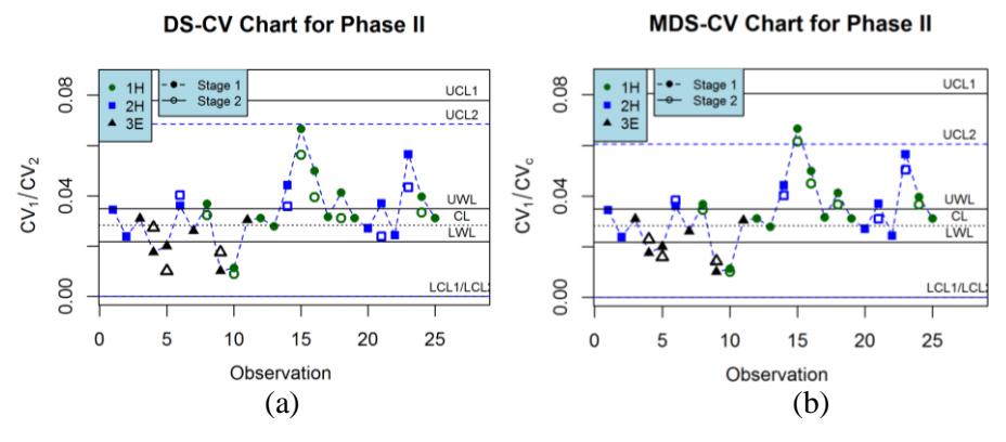
Figure 8 Monitoring CV for the Phase II data set with \(n_1 = 3\) and \(n_2 = 3\), using (a) the DS-CV chart and (b) the MDS-CV chart. Based on the DS-CV chart, no OC signal was detected, while the OC signal was detected at the 15<sup>th</sup> observation, based on the MDS-CV chart in the second stage.
Furthermore, with \(ASS_0 = 5\) and sample size \((n_1 = 3, n_2 = 3)\), we obtained that the optimal parameter values \((W, L_1, L_2)\) that minimize Eq. (14) for the DS-CV chart were (0.750, 5.721, 4.749) and for the MDS-CV chart were (0.751, 5.978, 3.752). The CV values from Phase II using the DS-CV and MDS-CV chart are plotted in Figure 8(a)-(b), respectively, where the solid markers denote the sample CV in Stage 1 while the hollow markers denote the sample CV in Stage 2. Based on the DS-CV chart, the OC signal was not detected for all observations, while the OC signal was detected at the 15th observation, based on the MDS-CV chart in Stage 2. This shows that performing the MDS-CV chart worked better than the DS-CV chart in detecting out-of-control signals.
6 Conclusion
This study developed a modified DS-CV chart, denoted as MDS-CV chart, by considering the combination of information from the first and the second sample to obtain the conclusion in the second stage. The optimization model proved that the MDS-CV chart outperformed the DS-CV chart based on the \(ARL_1\) term, especially if the total sample size is small. If the total sample size is large, then the performance of the MDS-CV chart is equal to that of the DS-CV chart, indicating that using the MDS-CV chart is more efficient for taking the sample size, both in time and cost. Thus, it can be recommended to be applied in industry. The study case on the quality of the steel molding process in heavy
equipment companies showed that performing the MDS-CV chart worked better than the DS-CV chart in detecting out-of-control signals. Furthermore, the case study also showed that controlling the variability of several (three) types of materials with different mean and standard deviations of carbon composition could be done simultaneously using the CV chart. This is due to the proportional relationship between the mean and standard deviation of their carbon composition, so that control can be done based on the size of the CV.
Acknowledgement
The authors would like to thank RISTEK/BRIN Indonesia and PPMI FMIPA ITB 2023 for funding this research, and PT. Komatsu Indonesia (PT. KI) for the supplementary data. We also thank the anonymous reviewers for providing constructive comments to improve this version of the manuscript.
Nomenclature
| α | = | Probability of a type-I error |
|---|---|---|
| γ | = | Population (process) CV |
| \(\gamma_{\rm o}\) | = | In-control process CV |
| \(\gamma_1\) | = | Out-of-control process CV |
| τ | = | Shift size in the CV, \(\tau = \gamma_1/\gamma_0\) |
| \(F_G(.)/F_{G_c}(.)\) | = | Cumulative distribution function of \(G/G_c\) |
| \(F_G^{-1}(.)\) | = | Inverse cumulative distribution function of G |
| \(F_T(. | v, \delta)\) | = | Cumulative distribution function of non-central t-students |
| distribution with degree of freedom is \(v\) and parameter of non- | ||
| centrality is \(\delta\) | ||
| \(F_T^{-1}(. | v, \delta)\) | = | Inverse cumulative distribution function of non-central t-students |
| distribution with parameter of non-centrality is \(\delta\) and degree of | ||
| freedom is \(v\). | ||
| G | = | Sample CV |
| \(G_c\) | = | Combined sample CV |
| \(G_0\) | = | In-control process CV |
| n | = | Sample size |
| \(n_0\) | = | Desired value of ASS |
| Tr 1 | ||
| \(n_1\) | = | First sample size |
| \(n_1 \\ n_2\) | = | Second sample size |
| - | • | |
| \(n_2\) | = | Second sample size |
| \(n_2 \\ m\) | = | Second sample size Number of in-control Phase I samples |