
1 Introduction
NGC 6572 is among the brightest planetary nebulae (PNe) in the night sky. It makes the observation of the PN quite easy in terms of instrumental requirements, i.e., one can make use of a small-class telescope to obtain data with an adequate signal-to-noise ratio (SNR). Therefore, NGC 6572 is a PNe that has already been studied extensively. It not only shows typical PNe characteristics; several studies
Received August 6 th , 2023, Revised November 2 nd, 2023, Accepted for publication December 6 th, 2023 Copyright © 2023 Published by ITB Institut for Research and Community Service, ISSN: 2337-5760, DOI: 10.5614/j.math.fund.sci.2023.55.2.2math
have revealed that NGC 6572 has variability in its brightness and in the intensity of its nebular emission lines and stellar spectra. This indicates that NGC 6572 possesses an internal activity such that it affects its nebular brightness and spectral features.
Hyung et al. [1] investigated the variability of NGC 6572 using detailed highresolution spectra in the optical wavelength from 3650 to 10050 Å and highdispersion mode ultraviolet (UV) spectra from the International Ultraviolet Explorer (IUE) satellite. Hyung et al. [1] found that the central star of NGC 6572 may have a cycle of the order of 70 years. Miranda et al. [2] investigated the morphology of NGC 6572 using high-resolution images and reported that it possesses a point-symmetric feature that is enveloped within a previously known elliptical structure. Using high-resolution long-slit spectra, Miranda et al. [2] found the existence of highly collimated outflows, which may take part in the formation of the point-symmetric signature.
In this work, we report our long-slit spectroscopic observations at intermediate and low resolutions. We were able to obtain the recombination lines of H, Hβ, and He 6678 Å in the intermediate-resolution spectra. We also obtained several forbidden lines of [OIII] 4959 Å, [OIII] 5007 Å, [NII] 6548 Å, [NII] 6584 Å, [SII] 6716 Å, and [SII] 6731 Å. Forbidden lines in PNe spectra are useful to help investigate the nature of a PNe, e.g., nebular electron temperature and electron density, which are required to derive its nebular chemical composition. Different lines correspond to different ionization layers in the nebula, along with differences in their physical properties. Particularly for [OIII] and [NII], the emission lines can be used to constrain the temperature of the central star of planetary nebulae (CSPN).
We utilized the intermediate-resolution spectra to calculate the nebular expansion velocities and investigate its kinematical characteristics. In addition to that, the low-resolution spectra, covering the wavelengths from 3800 Å to 7700 Å, were used to derive the physical and chemical properties of the PN. The lines present in the spectra were employed as a constraint in the photoionization modeling, to make sure that the model could approximate the observed data to a certain degree of satisfaction.
2 Observations and Data Reductions
2.1 Intermediate-Resolution Spectra
We successfully secured two intermediate-resolution spectra taken on 14 June and 10 August 2021. Both spectra were obtained using a spectrograph mounted on a 10-inch (F/9.8) telescope with a CCD camera at Bosscha Observatory ITB,
Indonesia. The spectrograph was operated with a grating of 1200 grooves/mm and a slit with a width of 25 µm. Using these instruments, NGC 6572 was observed with an exposure time of 2700 seconds on 14 June and 3600 seconds on 10 August. During both observations the slit was centered on the object at a position angle (PA) of 0°.
We cleaned the spectrograms (subtracted them from biases, darks, and corrected the normalized flat) and performed spectra extraction (including wavelength and flux calibration) using long-slit IRAF (Image Reduction and Analysis Facility) routines. A Fe-Ne-Ar lamp was used as the calibration lamp to obtain wavelength calibration frames. The final spectra had a resolution of R~5000 and a spectral linear dispersion of 0.34 Å/pixel. The spectral wavelength coverages were from 4810-5090 ÅÅ for the 14 June observation and 6475-6740 ÅÅ for 10 August observation. Therefore, we obtained emission lines at Hβ, [OIII] 4959 Å, [OIII] 5007 Å, Hα, [NII] 6548 Å, [NII] 6584 Å, HeI 6678 Å, [SII] 6716 Å, and [SII] 6731 Å.
2.2 Low-Resolution Spectra
We also obtained low-resolution spectra to determine and analyze the chemical properties of NGC 6572. On 10 July 2022, we observed NGC 6572 using a fast and low-resolution long-slit spectrograph (Malasan et al. [3]) mounted on an 11 inch (F/10) telescope with a CCD camera at Bosscha Observatory ITB, Indonesia. With an exposure time of 300s, the slit was centered on the object at 0° PA. Data reduction was carried out in the same manner as for the intermediateresolution spectra, including the calibration lamp that was used. The procedure resulted in a spectrum with a resolution of R~1000, covering a wavelength range of 3875-7760 ÅÅ and with a spectral linear dispersion of 2.88 Å/pixel.
3 Nebular Kinematics
To analyze the nebular kinematics, we present the spectral images as well as the position-velocity (PV) contour maps in Figure 1. The PV maps were constructed from the reduced spectrograms of the intermediate-resolution spectra, where we converted the horizontal axis from wavelength into velocity using Doppler shift, with laboratory wavelengths as the reference. The spectral resolution from full width at half-maximum (FWHM) was ~15 kms -1 and the spatial resolution was ~0.73/pixel. From the PV contour maps, we can see the elliptical nebular shell of NGC 6572, but there is no sign of prominent and well-separated emission peaks. This is likely caused by the insufficient resolution to detect such a feature in the spectral images.
With the given spectral resolution, the emission lines of each detected ion do not show the double-peaked feature but rather single and broad emissions. The nature of the object, i.e., a compact planetary nebula with high surface brightness, adds to the underlying reason for this lack of detection. Thus, to determine the nebular expansion velocity we assumed that the nebula is an expanding spherical shell of gas that produces emission lines that can be represented by a Gaussian distribution. This introduces a separation velocity (\(\Delta v^2\)) that corresponds to the part of the nebular shell that is approaching and receding towards the observer. The separation velocity, which reflects the intrinsic velocity of the expanding nebula, can be calculated by subtracting the observed velocity from the observed instrumental and thermal line (Eq. 1).
\[\Delta v^2 = v_{observed}^2 - v_{instrumental}^2 - v_{thermal}^2. \tag{1}\]
The comparison lamp line measurements provide the \(v_{\rm instrumental}\) (\(c \times \frac{\rm FWHM}{\lambda}\)). The instrumental line broadening (converted into velocity) of the lines H\(\alpha\), [NII], HeI, and [SII] was ~61 kms<sup>-1</sup>, while the instrumental line broadening for H\(\beta\) and [OIII] was ~60 kms<sup>-1</sup>. The thermal broadening (\(v_{\rm thermal}\)) corresponding to the elements H, He, O, N, and S, was 21.26 kms<sup>-1</sup>, 10.63 kms<sup>-1</sup>, 5.31 kms<sup>-1</sup>,5.68 kms<sup>-1</sup>, and 3.76 kms<sup>-1</sup>, respectively (Choi et al. [4]). In Table 1, we present the nebular expansion velocities from every detected line. We found that the expansion velocities derived from blue spectra (H\(\beta\) and [OIII]) were somewhat larger compared to those derived from red spectra (H\(\alpha\), [NII], HeI, and [SII]), while the red spectra expansion velocities were close to the typical expansion velocity of planetary nebulae (~14-25 kms<sup>-1</sup>).
This can also be seen from the more rounded shape of the spectral images and the PV diagram of the blue spectra compared to the red spectra. Miranda et al. [2] in 1999 suggested that NGC 6572 possesses two velocities, i.e., 17 kms<sup>-1</sup> and 50 kms<sup>-1</sup>, therefore, it is possible that during the observation on 14 June, we observed a nebular region that exhibits this velocity. This means that NGC 6572 possesses several expansion velocities, where we can infer that several episodes of nebular ejection occurred during the formation of NGC 6572. The more rounded shape of the blue region spectra could also be the subject of the location where the lines are produced. H\(\beta\) especially is related to a location close to the center of the nebula, hence the CSPN. At such a location, the nebula does not interact so much with its surrounding environment, allowing it to keep its spherical shape.
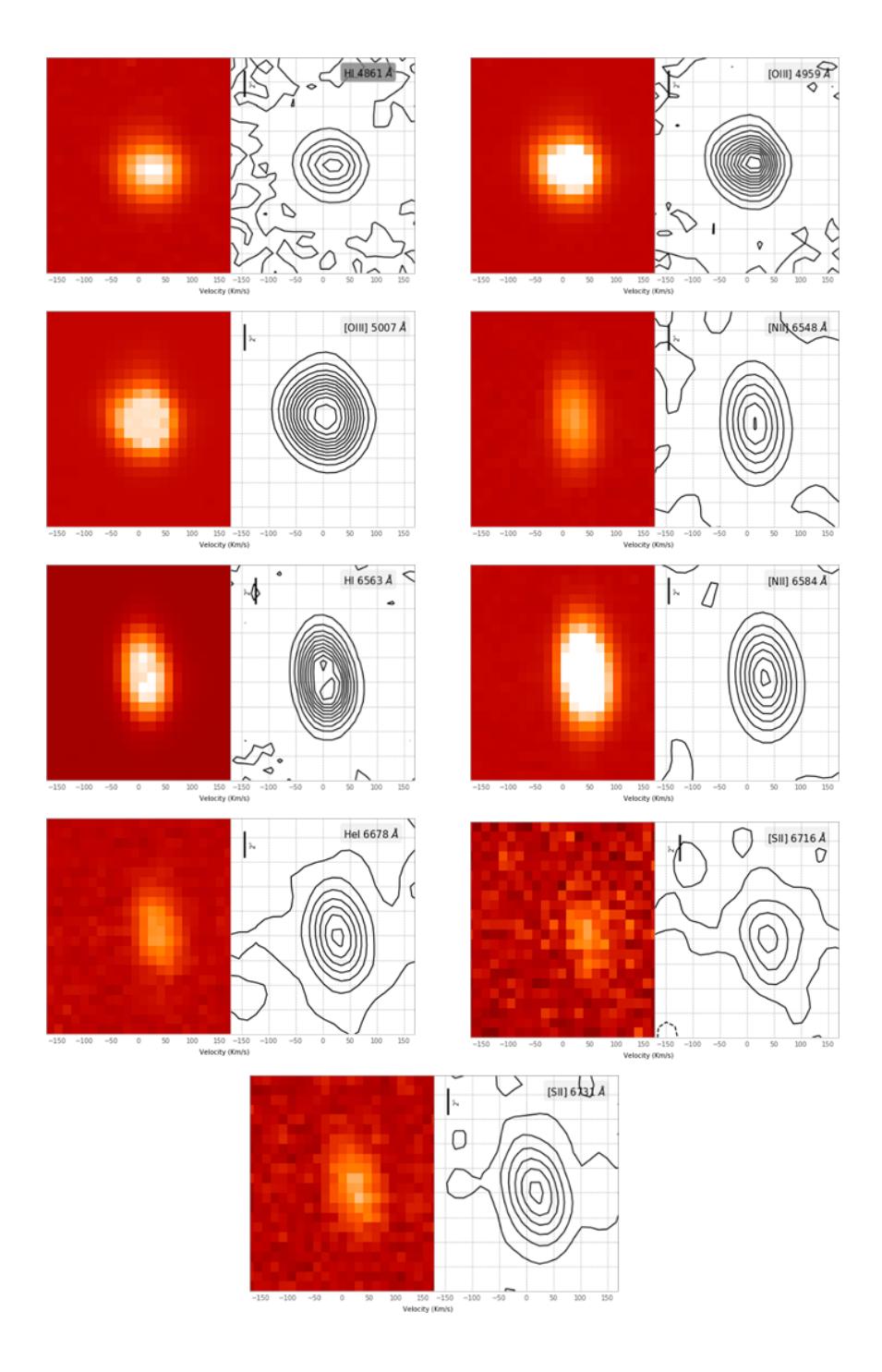
Figure 1 Spectral images and PV diagrams of the emission lines of NGC 6572.
| Ion | λ (Å) | vexp (kms-1 ) |
|---|---|---|
| Hβ | 4861.33 | 50.37 |
| Hα | 6562.82 | 15.22 |
| HeI | 6678.15 | 15.03 |
| [NII] | 6548.03 | 15.47 |
| 6583.45 | 16.73 | |
| [OIII] | 4958.92 | 48.31 |
| 5006.84 | 48.72 | |
| [SII] | 6716.16 | 17.76 |
| 6730.85 | 17.89 |
Table 1 Expansion velocity from several ions.
Table 2 presents the variation of the mean of the expansion velocity from the red spectra, as well as the ionization potential of each ion. PNe stratification implies that high excitation lines (from ions with high IP) are emitted at a location closer to the CSPN. Meanwhile, low excitation lines are emitted at a location further out from the CSPN. If the geometry is spherical, we should be able to see that the speed of the nebular gas expansion increases with the distance from the center (Wilson [5]). Since NGC 6572 is an ellipsoidal PN, there must be additional factors for the outward acceleration. The internal point-symmetric structure would likely contribute to this matter. From Table 2 we can also see that the measured velocities do not strictly follow the simple rule of a linear increasing velocity, given the increase in the ionization potential. This may also be caused by the internal structure that shapes the nebula.
Table 2 Expansion velocity vs ionization potential (IP).
| Ion | IP (eV) | vexp (kms-1 ) |
|---|---|---|
| [SII] | 10.4 | 17.82 |
| Hα | 13.6 | 15.22 |
| [NII] | 14.5 | 16.10 |
| HeI | 24.6 | 15.03 |
4 Nebular Properties
The intensity of the emission lines from the low-resolution spectrum were measured and used to deduce the nebular physical properties. We used NEAT (Nebular Empirical Analysis Tool) code [6] to determine the electron temperature and electron density from standard diagnostics. The code requires measured line fluxes, which are then corrected based on the interstellar extinction using the ratios of the intensity of the Balmer lines. The code was also used to calculate the ionic abundances from the flux-weighted averages of the emission lines of each
species. The total elemental abundances were calculated by incorporating an ionization correction factor (ICF). In this work, we applied the Howarth extinction law [7] for the interstellar extinction correction, and we used the ICF scheme from Delgado-Inglada et al. [8].
| Table 3 | Nebular physical properties. |
|---|
| c(Hβ) | Log FHβ | Te [NII] | Te [OIII] | Te [ArIII] | Ne [SII] | (N1+N2 [OIII])/H b | |
|---|---|---|---|---|---|---|---|
| This work | 0.37 | -11.33 | 12200 K | 10900 K | 9400 K | 3400 K | 19.56 |
| Hyung et al.[1] | 0.40 | -9.82 | 11000 K | … | … |
The nebular properties we derived are summarized in Table 3. The reddening, c(Hβ), and electron temperature from collisionally-excited lines were in relatively good agreement with the values from Hyung et al. [1]. We also found logFHβ and the density diagnostic from [SII] to be 0.37 and 3400 K, respectively. The line strength of 19.56 indicates that NGC 6572 has a moderate line strength, which means that the CSPN of NGC 6572 has a relatively moderate temperature and luminosity for a white dwarf star.
The elemental abundances (Table 4) calculated from the available emission lines were mostly lower than those from Hyung et al. [1], which may be caused by the limited number of emission lines that were taken into account in the calculation of the ionic abundances. The overall discrepancy from values determined by other researchers is subject to various aspects, e.g., a different nebular region observed as well as the data processing and calculation of physical properties procedures could have contributed to the departure from the resulted values.
Table 4 Nebular elemental abundances (log X/H) measured in this work and Hyung et al. [1].
| Element | This work | Hyung et al. [1] |
|---|---|---|
| N | -4.05 | -4.208 |
| O | -3.28 | -3.463 |
| Ne | -4.15 | -4.244 |
| Ar | -5.51 | -5.724 |
| S | -5.81 | -5.666 |
| Cl | -6.79 | -7.171 |
| He | -0.82 | 0.0044 |
4.1 Photoionization Model
Calculating nebular physical properties and elemental abundances using an empirical method is limited by the availability of emission lines in the spectra. A theoretical model of the nebular ionization structure constructed through photoionization modeling can provide more complete data and information of the lines emitted by the nebula. We employed the photoionization code Cloudy (version 17.02, [9]) to construct a self-consistent nebular structure.
Cloudy utilizes a set of input parameters that define the ionizing source as well as the nebula and then solves the ionization balance and energy balance equations at each point of the nebula. The code calculates the radiation transfer and generates the model spectrum at the end. The emitted spectra of the model then can be compared to the ones found in the observation.
| Central star | ||||
|---|---|---|---|---|
| Teff | 59979 K | |||
| log g | 4.2 | |||
| logL/L⊙ | 36.75 | |||
| Nebula | ||||
| Geometry | Sphere | |||
| logNH | 4.01 cm-3 | |||
| log r | 17.19 cm | |||
| Density | −2 𝑁0(𝑟/𝑟0) | |||
| Abundances (logX/H) | ||||
| N | -4.05 | |||
| O | -3.28 | |||
| Ne | -4.15 | |||
| Ar | -5.51 | |||
| S | -5.81 | |||
| Cl | -6.79 | |||
| He | -0.82 | |||
The input parameters listed in Table 5 consist of parameters regarding the ionizing source (CSPN), the nebular physical description, and the initial nebular chemical abundances that were previously determined empirically. The ionizing source is characterized with the SED from the stellar atmosphere that is defined by its luminosity, temperature, and gravity, all in a grid of stellar atmosphere models adopted from Hubeny [10].
The nebular parameters included the description of its geometry, density, radius, and chemical abundances. The spherical geometry was adopted so that the ionizing source would be located at the center of the nebula, and we did not employ a realistic complex geometry. The density was taken from the electron density with a decreasing distribution profile with a factor of -2. The initial elemental abundances were set to the values calculated previously using an empirical method.
To achieve the best-fitted model, we treated the density, radius, and the abundances as free parameters and varied them until the observables were satisfactorily reproduced by the model. Thus, the code will adjust for the line strength of different elements. Goodness of fit was obtained by calculating the root mean square (RMS) value using Eq. (2).
\[RMS = \sqrt{\frac{1}{N} \sum_{i} \left[1 - \frac{M_i^2}{o_i}\right]} \,. \tag{2}\]
\(M_i\) and \(O_i\) are the modeled and observed values of the i-th observable and N denotes the total number of observables. The model is considered acceptable if the RMS is less than unity.
The comparison between the observed and the modeled parameters are given in Table 6. The observed parameters are lines measured from the spectra and have been dereddened, and the electron temperature was calculated from the [OIII] lines. From the model, we obtained the line intensities of various ions that were not detected in the observation. The RMS calculation was based on the lines measured in the observation, and the RMS value was found to be quite far below unity.
The measured emission lines from the low-resolution spectra were close to those measured by Hyung et al. [1] but there were still differences in the intensities, especially on the edge of the spectra. The photoionization model on the other hand was mostly successful in generating spectra close to the observed lines. Discrepancies in the modeled spectra were also apparent, especially at lines that were not available in the observations. This was somewhat expected, since we did not provide constraints apart from the lines observed in the optical spectra and in our case the code could not successfully generate the lines to be close to those measured by Hyung et al. [1].
The elemental abundances resulted from the modeling are presented in Table 7. The values were still lower than those measured by Hyung et al. [1]. This could indicate that the nebula had undergone changes, especially compared to the previous study Hyung et al. [1]. It may also be a sign of the spectral variability apparent in nebula, but further investigation is needed to confirm this.
Table 6 Comparison of the measured line intensities from this work and Hyung et al. [1] and Cloudy model fit.
| Parameter | Obs. | Hyung et al. [1] (1) | Hyung et al. [1] (2) | Model |
|---|---|---|---|---|
| λ3727 | 16.88 | 13.25 | 246.85 | |
| λ3868 | 16.8 | 95.31 | 87.733 | 16.12 |
| λ4101 | 37.30 | 30.89 | 27.91 | 25.37 |
| λ4340 | 59.50 | 47.49 | 35.04 | 46.35 |
| λ4363 | 8.71 | 8.31 | 8.90 | 10.56 |
| λ4471 | 5.01 | 5.30 | 5.61 | 2.91 |
| λ4686 | 0.38 | 0.39 | 11.35 | |
| λ4740 | 2.26 | 2.48 | 1.00 | |
| λ5007 | 1530.00 | 1107.54 | 1077.36 | 1526.88 |
| λ5200 | 0.07 | 0.09 | 0.19 | |
| λ5518 | 0.16 | 0.17 | 0.99 | |
| λ5538 | 0.38 | 0.40 | 1.44 | |
| λ5755 | 2.16 | 1.46 | 1.71 | 0.78 |
| λ5876 | 15.80 | 16.93 | 16.66 | 8.46 |
| λ6300 | 9.82 | 3.05 | 3.82 | 30.95 |
| λ6312 | 4.81 | 0.66 | 0.80 | 0.31 |
| λ6563 | 359.00 | 307.54 | 280.48 | 292.06 |
| λ6584 | 37.39 | 44.64 | 40.89 | |
| λ6678 | 3.86 | 4.22 | 2.28 | |
| λ6717 | 0.53 | 0.47 | 1.94 | |
| λ6731 | 3.65 | 1.07 | 1.19 | 3.29 |
| λ7006 | 0.28 | 10.23 | 9.68 | 0.04 |
| λ7136 | 28.40 | 15.37 | 16.32 | 30.12 |
| T[OIII] | 10900 K | 11000 K | 10100 K | |
| RMS | 0.45 | |||
| λ1549 | 1.50 | 3.74 | ||
| λ1909 | >11.369 | 59.55 | ||
| λ2326 | 11.82 | 13.32 | ||
| λ9850 | 0.02 | 0.34 | ||
| λ1486 | 0.07 | |||
| λ1750 | 2.59 | 1.04 | ||
| λ2424 | 0.44 | |||
| λ8047 | 0.22 | 0.41 | ||
| λ9532 | 17.03 | 13.28 | 12.53 |
Note: The emission line strength is relative to Hβ = 100. (1) and (2) correspond to data collected in 1990 and 1991, respectively.
Element This work Hyung et al. [1] Model Sun N -4.05 -4.208 -4.6239 -4.17 O -3.28 -3.463 -3.1384 -3.31 Ne -4.15 -4.244 -4.6667 -3.94 Ar -5.51 -5.724 -5.5649 -5.62 S -5.81 -5.666 -6.0295 -4.88 Cl -6.79 -7.171 -6.6979 -6.69 He -0.82 0.0044 -1.1680 -1.086
Table 7 Comparison of the modeled chemical abundances in this work, Hyung et al. [1], and solar photospheric abundances (Asplund [11]).
5 Conclusions
From the intermediate-resolution long-slit spectra we can see an overall image of a nebular expansion pattern that corresponds to the ellipsoidal feature of the nebular morphology. The limited resolution of the observations hampered us to detect the internal point-symmetric structure as well as the collimated flows. Observations with higher resolution would provide a better image of the existing internal structure, while different slit orientations are needed to obtain the kinematics from another nebular region. The calculated expansion velocities are typical planetary nebulae expansion velocities for Hα, [NII] 6548 Å, [NII] 6584 Å, HeI 6678 Å, [SII] 6716 Å, and [SII] 6731 Å emission lines, but the value is somewhat higher for blue lines Hβ, [OIII] 4959 Å, and [OIII] 5007 Å. We suggest that the high velocity observed in the blue spectra may be a result of observing a different region within the nebula compared to the region observed in the red spectra. This, in turn, could indicate the presence of different velocity components in the nebula.
The nebular physical properties agree in terms of reddening and electron temperature, but differences in the measured line intensities appeared to affect the log FHβ and electron density. Several lines measured in our observation differed from those in Hyung et al. [1], which may suggest spectral variability in NGC 6572. By utilizing the measured lines and parameters from both the nebula and the CSPN, we successfully constructed a photoionization model with an RMS below unity. The overall chemical abundances, derived through both the empirical method and the photoionization model, were lower than those in Hyung et al. [1]. This difference may also indicate that the nebula may have evolved since Hyung et al. [1].
The complete kinematical maps with adequate resolution combined with high spatial resolution images can be further utilized to construct a 3D model of the nebula. Combining spatial and kinematical models with a photoionization model would produce a more comprehensive picture of the system. The complete picture of the nebula would allow for the deep investigation of the formation of the object.
Acknowledgements
This work was supported by the Faculty of Mathematics and Natural Sciences of Institut Teknologi Bandung (FMIPA ITB) under PPMI FMIPA ITB 2022 and PPMI KK Astronomy 2023. We also would like to thank Bosscha Observatory for providing the facilities to carry out this research.