Normal Form of Periodic FPU Chain of Four Particles with Alternating Masses

1 Introduction

In 1953, Enrico Fermi, John Robert Pasta, and Stanislaw Ulam (FPU) used the MANIAC-I computer to conduct a simulation of the vibration of 32 particles connected to each other with fixed endpoints. They introduced several nonlinear terms (quadratic, cubic, and piecewise linear) to the system and observed an unexpected result: for small initial energy, the system did not exhibit thermalization (i.e., the initial energy would be evenly distributed among all normal modes over time). Instead, it displayed an indication of quasi-periodic behavior (see the works of Fermi et al. in [1], Weissert in [2], Berman and Izrailev in [3], and Gallavotti in [4]). This surprising phenomenon motivated

Received July 3 rd, 2025, Revised September 24 th, 2025, Accepted for publication September 26th, 2025 Copyright © 2025 Published by ITB Institut for Research and Community Service, ISSN: 2337-5760, DOI: 10.5614/j.math.fund.sci.2025.57.1.4

many researchers to do further investigations and their results significantly contributed to the development of nonlinear wave theory.

Subsequent studies have explored modifications of the classical FPU chain. Instead of using fixed endpoints, one can consider the periodic chain, where the two endpoints are connected to each other. One of the remarkable results about this chain was established by Rink in [5], who analyzed its integrability and symmetries using the so-called Birkhoff-Gustavson normal form.

Another variation of the chain involves the mass distribution. While the classical chain assumes all masses to be 1 (homogeneous chain), recent researchers have studied inhomogeneous chains, where the masses vary arbitrarily, and alternating chains, where the system consists of 2 particles with alternating masses 1, , 1, , ⋯. The effects of mass variation on resonance phenomena in the inhomogeneous chain are studied by Bruggeman and Verhulst in [6] and by Hanßmann et al. in [7]. On the other hand, several works by Bruggeman and Verhulst in [8] and [9], Verhulst in [10], and van der Kallen and Verhulst in [11] explored interesting aspects of the alternating chain, such as the near-integrability and recurrence, and the interactions between the so-called optical and acoustic groups, using the averaging method.

Although higher-order averaging theory exists in principle (see Sanders et al. in [12]), its implementation is cumbersome and therefore rarely pursued in practice. As a consequence, averaging is typically carried out only up to the second order, yielding approximations accurate to ( 2 ). This limitation may also explain why previous works restricted their attention to quartic potentials in the Hamiltonian. Higher-order approximation can be done using the Birkhoff-Gustavson normal form, but this method is primarily used in studies of the integrability rather than the dynamics of the system.

What is new in this paper. We aim to explicitly show how Birkhoff-Gustavson normalization can be used to study the dynamics of a Hamiltonian system. In particular, we apply certain procedures to the alternating FPU chain with a general potential function, thereby enabling the study of this classical system in a broader and more flexible setting than previously considered. Specifically, we focus on studying the case of 4 particles. This model is important, since the dynamics of this system appear also in the phase space of chains with multiples of 4 masses. Bruggeman and Verhulst in [8] stated this as Theorem 3.1. Thus, insights obtained from the four-particle case are directly relevant to the understanding of larger systems.

1.1 Outline

In Section 2 and 3, we present the mathematical formulation of Hamiltonian systems and also the theoretical framework of Birkhoff-Gustavson normalization. In particular, we show how an appropriate choice of coordinate system simplifies the normalization process due to the structure of the transformed Hamiltonian.

Section 4 introduces the mathematical formulation of an alternating FPU chain consisting of four particles with masses 1, m, 1, m. By applying the symplectic transformation introduced by Hanßmann et al. in [7], the Hamiltonian becomes independent of one coordinate due to the existence of a momentum integral, which allows a reduction of one degree of freedom. Furthermore, the resulting Hamiltonian takes a semi-simple form and exhibits three discrete symmetries.

In Section 5, we present a detailed step-by-step procedure on how to do further analysis using Birkhoff-Gustavson normalization. We demonstrate the procedure for two values of \(\mu = \frac{1}{m}\). The first is \(\mu = 1\) (homogeneous chain), whose normal form leads to a system of oscillators with frequency ratio \(\sqrt{2}\): 1: 1, and the second is \(\mu = 3\), where it corresponds to the ratio 2: 1: \(\sqrt{3}\). These include 'sub-resonances' 1: 1 and 2: 1, which are the most prominent resonances. For each case, we construct the Birkhoff-Gustavson normal form and show that, in action-angle variables, it possesses two conserved quantities and depends on only one angular coordinate. Consequently, the system can be reduced to a single degree of freedom. This enables us to do a qualitative analysis in symplectic Cartesian coordinates and uncover dynamical behaviors analogous to resonance phenomena observed in celestial mechanics and other areas of physics (see Pousse and Alessi in [13], Huang et al. in [14], Li et al. in [15], and Dam et al. in [16]).

2 Hamiltonian Systems

Consider the vector space \(\mathbb{R}^{2n}\) with coordinate \(\mathbf{v} = (\mathbf{q}, \mathbf{p})^T\) where \(\mathbf{q}, \mathbf{p} \in \mathbb{R}^n\) as symplectic linear space, i.e., a vector space equipped with a non-degenerate symplectic form:

\[\boldsymbol{q} \wedge \boldsymbol{p} = \sum_{1}^{n} (dq_{j} \wedge dp_{j}). \tag{1}\]

Let us denote by D a differential operator:

\[D \coloneqq \left(\partial_{q_1}, \dots, \partial_{q_n}, \partial_{p_1}, \dots, \partial_{p_n}\right)^T.\]

Suppose \(H: \mathbb{R}^{2n} \to \mathbb{R}\) is a real analytic function. A Hamiltonian system of ordinary differential equations is defined by:

\[\dot{\mathbf{v}} := \frac{d}{dt} \mathbf{v} = J DH \equiv X_H(\mathbf{v}), \tag{2}\] where

\[J = \begin{pmatrix} 0 & I_n \\ -I_n & 0 \end{pmatrix}\] with \(I_n\) is the \(n \times n\) identity matrix. The function H is called the Hamiltonian function and \(X_H\) is called the Hamiltonian vector field corresponding to H.

Let \(\mathcal{F}\) be a linear space of real analytic functions. On \(\mathcal{F}\), the symplectic form (1) induces a bracket, i.e., the (standard) Poisson bracket:

\[\{f,g\} = (Df)^T J(Dg) = \sum_{j=1}^n \left( \partial_{q_j} f \cdot \partial_{p_j} g - \partial_{p_j} f \cdot \partial_{q_j} g \right).\]

This bracket is bi-linear and skew symmetric \((\{f,g\} = -\{g,f\})\). Using this bracket, the Hamiltonian system (2) can be written as:

\[\begin{cases} \dot{q}_j = \{q_j, H\} \\ \dot{p}_j = \{p_j, H\} \end{cases}\] where \(j = 1, 2, \dots, n\). A function \(F: \mathbb{R}^{2n} \to \mathbb{R}\) is called an integral of (2) if it is constant along the solution, i.e.,

\[0 = \frac{d}{dt}F(\mathbf{v}(t)) = (DF)\dot{\mathbf{v}} = (DF)J(DH) = \{F, H\}.\]

In this case, we say that F is Poisson commute with H.

3 On Normalization

Let \(\mathcal{P}_k\) be the space of homogeneous polynomials of degree k in variables \(\boldsymbol{\nu}\), i.e.,

\[\mathcal{P}_k \coloneqq \operatorname{span}_{\mathbb{R}} \{ q_1^{k_1} \cdots q_n^{k_n} p_1^{k_{n+1}} \cdots p_n^{k_{2n}} | \sum_{j=1}^{2n} k_j = k \},\] and let \(\mathcal{P}\) be the space of all convergent series \(\sum_{j=1}^{\infty} \alpha_{j} p_{j}\), where \(p_{j} \in \mathcal{P}_{j}\). With an abuse of notation, we may write \(\mathcal{P} = \bigoplus_{k \geq 2} \mathcal{P}_{k}\). We have equipped \(\mathcal{P}\) with the standard Poisson bracket as defined in the previous section.

Let us consider an arbitrary element \(h \in \mathcal{P}\). To it, we associate a linear operator \(\mathrm{ad}_h \colon \mathcal{P} \to \mathcal{P}\) by setting: \(\mathrm{ad}_h(f) = \{h, f\}\). It is easy to see that whenever \(h \in \mathcal{P}_k\), then \(\mathrm{ad}_h \colon \mathcal{P}_\ell \to \mathcal{P}_{k+\ell-2}\). In particular, if \(h \in \mathcal{P}_2\), then \(\mathrm{ad}_h \colon \mathcal{P}_\ell \to \mathcal{P}_\ell\).

Furthermore, for that arbitrary h, let us consider the Hamiltonian vector field \(X_h\). For an open neighborhood U of the origin of \(\mathbb{R}^{2n}\), we denote by \(\exp(tX_h): U \to \mathbb{R}^{2n}\) the time t-flow of the Hamiltonian system of differential equations (2). This flow defines a symplectic diffeomorphism on U, whenever \(t \in [-1,1]\).

Lemma 1. If \[H, h \in \mathcal{P}\], then \(H \circ \exp(-X_h) = \exp(\operatorname{ad}_h) H\)

Proof. For arbitrary \(t \in [-1,1]\) and \(f \in \mathcal{P}\), consider the curve in \(\mathcal{P}\), which is defined by \(\gamma(t) = f(\exp(tX_h))\). Note that:

\[\frac{d\gamma}{dt} = (Df)(\exp(tX_h))^T \frac{d}{dt} \exp(tX_h)\] \[= (Df)(\exp(tX_h))^T (JDh)\] \[= \{f(\exp(tX_h)), h\}\] \[= -\mathrm{ad}_h(\gamma)\] which is a linear differential equation in \(\mathcal{P}\). Taking the initial condition: \(\gamma(0) = f\), the solution reads \(\gamma(t) = \exp(-t \cdot \operatorname{ad}_h)f\). The proof is completed by choosing t = -1 and f = H. \(\square\)

Note that we can view \(\exp(-X_h)\): \(U \to \mathbb{R}^{2n}\) as a symplectic coordinate transformation, since it is a symplectic diffeomorphism on U to its image, which defines a coordinate transformation. Using this, we can transform the Hamiltonian system of ordinary differential equations (2) to another system of ordinary differential equations. Since this coordinate transformation is symplectic, it preserves the symplectic form, so that the transformed system stays Hamiltonian, with the following Hamiltonian function:

\[\mathcal{H} = H(\exp(-X_h)) = \exp(\mathrm{ad}_h)H. \tag{3}\]

Suppose \(\mathcal{H}\) is the Hamiltonian of the transformed system. Then it is exactly the original Hamiltonian function evaluated at the new coordinate as in (3), i.e.,

\[\mathcal{H} = \exp(\mathrm{ad}_h)H\]
= \(\left(I + (\mathrm{ad}_h) + \frac{1}{2!}(\mathrm{ad}_h)^2 + \cdots\right)H\)

\[= H + \{h, H\} + \frac{1}{2!} \{h, \{h, H\}\} + \cdots.\]

Furthermore, if \(h \in \bigoplus_{k\geq 3} \mathcal{P}_k\), then the derivative \(D(\exp(-X_h))\) at the origin is the identity transformation, i.e., it is a near identity transformation.

Let us now write \(H = H_2 + H_3 + H_4 \cdots\), where \(H_k \in \mathcal{P}_k\). Similarly, the function h is written as \(h = h_3 + h_4 + \cdots\), where \(h_k\) are to be determined. Then

\[\mathcal{H} = H_2 + (H_3 + \{h_3, H_2\}) + \left(H_4 + \{h_3, H_3\} + \frac{1}{2!} \{h_3, \{h_3, H_2\}\} + \{h_4, H_2\}\right) + \cdots\] (4)

One can start by looking at the third order term, i.e., \((H_3 + \{h_3, H_2\})\), or similarly:

\[\mathcal{H} = H_3 + \{h_3, H_2\} = H_3 - \operatorname{ad}_{H_2}(h_3).\]

Here, we can write \(H_3\) as the sum \(H_3' + H_3''\), where \(H_3'\) are in the image of the linear operator \(\mathrm{ad}_{H_2}\). As a consequence, we can choose \(h_3\) such that \(\mathrm{ad}_{H_2}(h_3) =\)\(H_3'\). By doing this, (4) becomes: \(\mathcal{H} = H_2 + H_3^r + (\overline{H}_4 - \operatorname{ad}_{H_2}(h_4)) + \cdots\)where: \(\overline{H}_4 = (H_4 + \{h_3, H_3\} + \frac{1}{2!} \{h_3, \{h_3, H_2\}\})\). Obviously, all the higherorder terms need to be adjusted due to the choice of \(h_3\). Similarly, we split \(\overline{H}_4\)into \(\overline{H}_4' + \overline{H}_4''\). We proceed by solving

\[\operatorname{ad}_{H_2}(h_4) = \overline{H}_4'.\]

We can go on up to any desired degree. Suppose that we have chosen \(h_{k-1}\), then the transformed Hamiltonian is:

\[\mathcal{H} = H_2 + H_3^r + \dots + \overline{H}_{k-1}^r + \overline{H}_k + \dots\]

By solving the so-called homological equation,

\[\operatorname{ad}_{H_2}(h_k) = (\overline{H}_k)',\]

we define \(h_k\).

Resonance Analysis 3.1

Suppose that the quadratic part of the Hamiltonian is semi-simple, i.e.,

\[H = \frac{1}{2} \sum_{j=1}^{N} \omega_j \left( p_j^2 + q_j^2 \right) + H_3(\mathbf{v}) + \cdots\] (5)

where \(\omega_j\) are positive real numbers and \(H_k\) is a homogeneous polynomial of degree k. Let us transform the coordinate to \((\mathbf{a}, \mathbf{b})\) by defining

\[a_j = \frac{1}{\sqrt{2i}} (p_j + iq_j), b_j = \frac{1}{\sqrt{2i}} (p_j - iq_j), i^2 = -1, j = 1, 2, \dots, N.\] (6)

This transformation is symplectic; thus, it preserves the symplectic structure. The quadratic term of the transformed Hamiltonian now becomes \(H_2 = i \sum_{j=1}^{N} \omega_j \, a_j b_j\).

In this coordinate, the operator \((ad_{H_2})\) acts diagonally on \(\mathcal{P}\). Indeed, consider the monomial

\[f = \delta \prod_{j=1}^{N} a_j^{\alpha_j} b_j^{\beta_j}\], with \(\sum_{j=1}^{N} \alpha_j + \beta_j = k\).

Then

\[\operatorname{ad}_{H_2}(f) = i \sum_{j=1}^{N} ((\beta_j - \alpha_j)\omega_j) f.\]

In this new coordinate, it becomes very clear that the space \(\mathcal{P}_k\) for \(k=2,3,\cdots\) is split into the sum \(\operatorname{Ker}(\operatorname{ad}_{H_2})+\operatorname{Im}(\operatorname{ad}_{H_2})\). Since we can transform away everything that is in the image, we conclude that a monomial f is in the normal form if it is in \(\operatorname{Ker}(\operatorname{ad}_{H_2})\). Furthermore, the monomial f is in \(\operatorname{Ker}(\operatorname{ad}_{H_2})\) if and only if

\[\sum_{j=1}^{N} \left( (\beta_j - \alpha_j) \omega_j \right) = 0.\]

This relation is also known as the resonance relation.

If \(f \in \text{Im}(\text{ad}_{H_2})\), we may choose

\[\frac{1}{\mathrm{i} \sum_{j=1}^N \left( (\beta_j - \alpha_j) \omega_j \right)} f\] as a normalizing term in \(h_k\) to remove the corresponding monomial from the transformed Hamiltonian.

Lemma 2. There exists a near identity symplectic coordinate transformation that transforms the Hamiltonian H in (5) into \(\mathcal{H}\), which is truncated up to degree n, which is Poisson commute with \(H_2\).

The truncation implies that we end up with an approximation of the original Hamiltonian system. This approximation, however, is improved because it has an extra integral of motion.

4 Formulation of FPU Chain

Let \(q_j\) be the displacement of each particle and \(p_j\) be the momentum. The periodic FPU chain of 4 particles with alternating masses has a Hamiltonian function

\[H(q, p) = \sum_{j=1}^{4} \left( \frac{1}{2m_j} p_j^2 + V(q_{j+1} - q_j) \right)\] (7)

where \(m_1 = m_3 = 1\), \(m_2 = m_4 = m > 0\). We apply the periodicity condition, i.e., \(q_5 = q_1\). The potential function V chosen in this paper is:

\[V(z) := \frac{1}{2}z^2 + \frac{\rho_1}{3}z^3 + \frac{\rho_2}{4}z^4 + \frac{\rho_3}{5}z^5 + \frac{\rho_4}{6}z^6 + \cdots,\] where \(\rho_j\) are parameters. One can see this potential function as a generic analytic function in its variable.

Using this Hamiltonian, we derive the equations of motion in the usual way. Then the linear part of the equations of motion can be written as \(\ddot{q} + ACq = 0\) where \(A = \text{diag}(1, \mu, 1, \mu)\) with \(\mu = 1/m\) and

\[C = \begin{bmatrix} 2 & -1 & 0 & -1 \\ -1 & 2 & -1 & 0 \\ 0 & -1 & 2 & -1 \\ -1 & 0 & -1 & 2 \end{bmatrix}.\]

Following Hanßmann et al. in [7], we define a symplectic transformation:

\[q = A^{1/2}U\Omega^{-1/4}\mathbf{Q}\] and \(p = A^{-1/2}U\Omega^{1/4}\mathbf{P}\), (8)

with \(\Omega=\mathrm{diag}(\omega_1,\omega_2,\omega_3,1),\) where \(\omega_1=\sqrt{2\mu+2},\) \(\omega_2=\sqrt{2},\) \(\omega_3=\sqrt{2\mu},\) and

\[U = \begin{bmatrix} -\frac{1}{\sqrt{2\mu+2}} & -\frac{1}{\sqrt{2}} & 0 & \frac{\sqrt{\mu}}{\sqrt{2\mu+2}} \\ \frac{\sqrt{\mu}}{\sqrt{2\mu+2}} & 0 & -\frac{1}{\sqrt{2}} & \frac{1}{\sqrt{2\mu+2}} \\ -\frac{1}{\sqrt{2\mu+2}} & \frac{1}{\sqrt{2}} & 0 & \frac{\sqrt{\mu}}{\sqrt{2\mu+2}} \\ \frac{\sqrt{\mu}}{\sqrt{2\mu+2}} & 0 & \frac{1}{\sqrt{2}} & \frac{1}{\sqrt{2\mu+2}} \end{bmatrix}.\]

This transformation brings the quadratic part of (7) into:

\[H_2 = \sum_{j=1}^{3} \frac{\omega_j}{2} (P_j^2 + Q_j^2) + \frac{1}{2} P_4^2.\] (9)

Note that the Hamiltonian does not depend on ⁴ due to the conservation of momentum. Therefore, we can reduce the dimension by omitting (4,4). The complete formula for reads:

\[\begin{split} H &= \frac{\omega_{1}}{2} \left( P_{1}^{\ 2} + Q_{1}^{\ 2} \right) + \frac{\omega_{2}}{2} \left( P_{2}^{\ 2} + Q_{2}^{\ 2} \right) + \frac{\omega_{3}}{2} \left( P_{3}^{\ 2} + Q_{3}^{\ 2} \right) - \\ &\rho_{1} \omega_{1} \omega_{2} \omega_{3} Q_{1} Q_{2} Q_{3} + \frac{\rho_{2}}{16} \left( \omega_{1}^{\ 2} Q_{1}^{\ 4} + \omega_{2}^{\ 2} Q_{2}^{\ 4} + \omega_{3}^{\ 2} Q_{3}^{\ 4} \right) + \\ &\frac{3\rho_{2}}{8} \left( \omega_{1} \omega_{2} Q_{1}^{\ 2} Q_{2}^{\ 2} + \omega_{1} \omega_{3} Q_{1}^{\ 2} Q_{3}^{\ 2} + \omega_{2} \omega_{3} Q_{2}^{\ 2} Q_{3}^{\ 2} \right) - \\ &\frac{\rho_{3}}{2} \left( \sqrt{\omega_{1}^{\ 3} \omega_{2} \omega_{3}} Q_{1}^{\ 3} Q_{2} Q_{3} + \sqrt{\omega_{1} \omega_{2}^{\ 3} \omega_{3}} Q_{1} Q_{2}^{\ 3} Q_{3} + \\ &\sqrt{\omega_{1} \omega_{2} \omega_{3}^{\ 3}} Q_{1} Q_{2} Q_{3}^{\ 3} \right) + \rho_{4} \left( \frac{1}{96} \left( \omega_{1}^{\ 3} Q_{1}^{\ 6} + \omega_{2}^{\ 3} Q_{2}^{\ 6} + \omega_{3}^{\ 3} Q_{3}^{\ 6} \right) + \\ &\frac{15}{16} \omega_{1} \omega_{2} \omega_{3} Q_{1}^{\ 2} Q_{2}^{\ 2} Q_{3}^{\ 2} \right) + \text{ higher-order terms.} \end{split} \tag{10}\]

One can check that this Hamiltonian admits three discrete symmetries:

\[\begin{split} S_1\colon &(-Q_1,-Q_2,Q_3,-P_1,-P_2,P_3) \mapsto (Q_1,Q_2,Q_3,P_1,P_2,P_3) \\ S_2\colon &(Q_1,-Q_2,-Q_3,P_1,-P_2,-P_3) \mapsto (Q_1,Q_2,Q_3,P_1,P_2,P_3) \\ S_3\colon &(-Q_1,Q_2,-Q_3,-P_1,P_2,-P_3) \mapsto (Q_1,Q_2,Q_3,P_1,P_2,P_3) \end{split}\]

5 Normal Form Analysis

The procedure is carried out as follows:

• 1. Given a fixed value of , we apply (8) to our original Hamiltonian. We then omit the variable 4, so that we have the semi-simple form (4).
• 2. Next, we transform the Hamiltonian using the change of variables in (6) and perform the Birkhoff-Gustavson normalization. We denote the resulting normal form by ℋ.
• 3. We then apply the action-angle transformation

\[\sqrt{\mathrm{i}} \ a_j = \sqrt{r_j} \exp(\mathrm{i}\theta_j), \quad \sqrt{\mathrm{i}} \ b_j = \sqrt{r_j} \exp(-\mathrm{i}\theta_j), \quad j = 1,2\] (11)

to the normalized Hamiltonian.

• 4. We identify first integrals in the system, allowing a further reduction in the number of variables. In the case studied here, two integrals are found. The resulting reduced system remains Hamiltonian; we denote its Hamiltonian function by ℋ′ .
• 5. Finally, we analyze the equilibria and phase portrait of the system derived from ℋ′ by transforming to Cartesian coordinates:

\[x = \sqrt{2R}\cos(\varphi), \quad y = \sqrt{2R}\sin(\varphi).\] (12)

5.1 Case \(\mu = 1\)

In this case, the ratio would be \(\sqrt{2}\): 1:1. Using the proposed procedure, the normal form up to order 4 would be \(\mathcal{H} = \mathcal{H}_2 + \mathcal{H}_4\) with

\[\mathcal{H}_2 = i(2a_1b_1 + \sqrt{2}a_2b_2 + \sqrt{2}a_3b_3)\] and

\[\mathcal{H}_{4} = \rho_{1}^{2} \left( \frac{\sqrt{2}}{2} a_{1} b_{1} a_{2} b_{2} + \frac{\sqrt{2}}{2} a_{1} b_{1} a_{3} b_{3} + \frac{1}{4} a_{2}^{2} b_{3}^{2} + \frac{1}{4} a_{3}^{2} b_{2}^{2} \right) -\] \[\rho_{2} \left( \frac{3}{8} a_{1}^{2} b_{1}^{2} + \frac{3}{16} a_{2}^{2} b_{2}^{2} + \frac{3}{16} a_{3}^{2} b_{3}^{2} + \frac{3}{4} \sqrt{2} a_{1} b_{1} a_{2} b_{2} + \right.\] \[\left. + \frac{3}{4} \sqrt{2} a_{1} b_{1} a_{3} b_{3} + \frac{3}{4} a_{2} b_{2} a_{3} b_{3} + \frac{3}{16} a_{2}^{2} b_{3}^{2} + \frac{3}{16} a_{3}^{2} b_{2}^{2} \right).\]

Applying (11) would lead us to:

\[\mathcal{H} = 2r_1 + \sqrt{2}(r_2 + r_3) - \frac{\sqrt{2}\rho_1^2}{2}(r_1r_2 + r_1r_3) + \frac{3\rho_2}{16}(2r_1^2 + r_2^2 + r_3^2) + \frac{3\rho_2}{4}(\sqrt{2}r_1r_2 + \sqrt{2}r_1r_3 + r_2r_3) - \frac{1}{8}(4\rho_1^2 - 3\rho_2)r_2r_3\cos\varphi,\] where \(\varphi = 2\theta_2 - 2\theta_3\). One can check that \(r_2 + r_3 = E_0 > 0\) is an integral. Moreover, this Hamiltonian does not depend on \(\theta_1\), so that \(r_1\) is also an integral. Thus, the variables involved can be reduced. If \(R = r_2\), one may derive a simplified system:

\[\begin{cases} \dot{R} = \left(\rho_1^2 - \frac{3}{4}\rho_2\right)R(E_0 - R)\sin\varphi \\ \dot{\varphi} = -\frac{3\rho_2}{4}(E_0 - 2R) + \left(\rho_1^2 - \frac{3\rho_2}{4}\right)(E_0 - 2R)\cos\varphi \end{cases}\]

This system is still a Hamiltonian system. If the Hamiltonian is denoted as \(\mathcal{H}'\), then the explicit expression of it in (12) is:

\[\text{[rumus tidak dapat ditampilkan dengan baik — lihat PDF asli]}\]

If \(\rho_2 = 0\), then the system derived from (13) would have five equilibria (see Figure 1): \((0,0), (\sqrt{E_0},0), (-\sqrt{E_0},0), (0,\sqrt{2E_0}), (0,-\sqrt{2E_0})\)

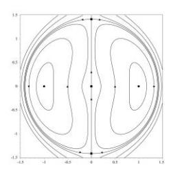
Figure 1 Phase portrait of the Hamiltonian system with Hamiltonian (13) with ² = 0, ¹ = 1, ⁰ = 1.

Now, if ² ≠ 0, one may divide (13) with ² and define a new parameter = ( 1 2 2 − 3 4 ), such that

\[\mathcal{H}' = -\frac{3}{16}(x^2 + y^2)^2 + \frac{3}{8}E_0(x^2 + y^2) - \frac{Cx}{4}\sqrt{x^2 + y^2}(2E_0 - (x^2 + y^2)).\] (14)

This system derived from (14) has the following properties (see Figure 2):

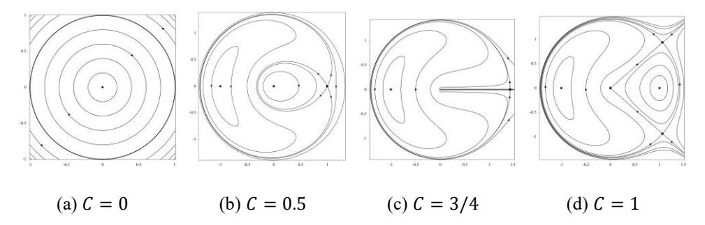
Figure 2 Phase portrait of the system derived from Hamiltonian (14) with ⁰ = 1.

• 1. The origin is an equilibrium point.
• 2. If = 0, the circle ² + ² = ⁰ is a manifold of equilibria (see Figure 2(a)).
• 3. There are other possible equilibrium points:

\[EP_{1} = (\sqrt{E_{0}}, 0), \qquad EP_{2} = (-\sqrt{E_{0}}, 0),\] \[EP_{3} = \left(\frac{3\sqrt{2E_{0}}}{4C}, \frac{\sqrt{2E_{0}(16C^{2} - 9)}}{4C}\right), \qquad EP_{4} = \left(\frac{3\sqrt{2E_{0}}}{4C}, -\frac{\sqrt{2E_{0}(16C^{2} - 9)}}{4C}\right).\]

• b. If || = 3/4, then there are three equilibrium points: 1,2, and = ³ = 4. It also has line (, 0) for > 0 as a manifold of equilibria (see Figure 2(c)).
• c. If || > 3/4, then the four equilibrium points exist and are all different (see Figure 2(d)).
• 6. It has a symmetry under transformation Ψ(, , 0, ) = (−, , 0, −), so that the phase portrait for < 0 is just a reflection over the -axis of the phase portrait for > 0.
• 7. If → ±∞, then ² → 0 and thus, the phase portrait will converge to Figure 1.

5.2 Case =

The ratio would be 2: 1:√3. The normal form up to order 6 would be ℋ = ℋ² + ℋ⁴ + ℋ⁶ with

\[\begin{split} \mathcal{H}_2 &= \mathrm{i} \left( \sqrt{8} a_1 b_1 + \sqrt{2} a_2 b_2 + \sqrt{6} a_3 b_3 \right), \\ \mathcal{H}_4 &= \rho_1^2 (a_1 b_1 a_2 b_2 + \sqrt{3} a_1 b_1 a_3 b_3) - \rho_2 \left( \frac{3}{4} {a_1}^2 {b_1}^2 + \frac{3}{16} {a_2}^2 {b_2}^2 + \frac{9}{16} {a_3}^2 {b_3}^2 + \frac{3}{2} a_1 b_1 a_2 b_2 + \frac{3\sqrt{3}}{2} a_1 b_1 a_3 b_3 + \frac{3\sqrt{3}}{4} a_2 b_2 a_3 b_3 \right), \end{split}\] and

\[\mathcal{H}_6 = i\rho_1^4 F_1 - i\rho_1^2 \rho_2 F_2 + i\rho_2^2 F_3 + i\rho_1 \rho_3 F_4 - \rho_4 F_5,\] where,

\[\text{[rumus tidak dapat ditampilkan dengan baik — lihat PDF asli]}\]

\[\begin{aligned} &\frac{9\sqrt{6}}{32}a_1{}^2b_1{}^2a_3b_3 + \frac{27\sqrt{2}}{8}a_1b_1a_3{}^2b_3{}^2 + \frac{99\sqrt{6}}{256}a_2{}^2b_2{}^2a_3b_3 + \\ &\frac{189\sqrt{2}}{256}a_2b_2a_3{}^2b_3{}^2 - \frac{33\sqrt{2}}{256}\left(a_1{}^2b_2{}^4 + a_2{}^4b_1{}^2\right), \\ &F_4 = 3\sqrt{2}a_1{}^2b_1{}^2a_2b_2 + \frac{3\sqrt{2}}{2}a_1b_1a_2{}^2b_2{}^2 + 3\sqrt{6}a_1{}^2b_1{}^2a_3b_3 + \\ &\frac{9\sqrt{2}}{2}a_1b_1a_3{}^2b_3{}^2 + 6\sqrt{6}a_1b_1a_2b_2a_3b_3 - \frac{3\sqrt{2}}{8}\left(a_1{}^2b_2{}^4 + a_2{}^4b_1{}^2\right), \text{ and } \\ &F_5 = \frac{5\sqrt{2}}{12}a_1{}^3b_1{}^3 + \frac{5\sqrt{2}}{96}a_2{}^3b_2{}^3 + \frac{5\sqrt{6}}{32}a_3{}^3b_3{}^3 + \frac{15\sqrt{6}}{4}a_1b_1a_2b_2a_3b_3 + \\ &\frac{15\sqrt{2}}{8}a_1{}^2b_1{}^2a_2b_2 + \frac{15\sqrt{2}}{16}a_1b_1a_2{}^2b_2{}^2 + \frac{15\sqrt{6}}{8}a_1{}^2b_1{}^2a_3b_3 + \\ &\frac{45\sqrt{2}}{16}a_1b_1a_3{}^2b_3{}^2 + \frac{15\sqrt{6}}{32}a_2{}^2b_2{}^2a_3b_3 + \frac{45\sqrt{2}}{32}a_2b_2a_3{}^2b_3{}^2 - \\ &\frac{5\sqrt{2}}{64}\left(a_1{}^2b_2{}^4 + a_2{}^4b_1{}^2\right). \end{aligned}\]

Applying (11) to the Hamiltonian, one may derive:

\[\dot{r}_1 = -\kappa r_1 r_2^2 \sin(2\theta_1 - 4\theta_2), \\ \dot{r}_2 = -2\dot{r}_1, \text{ and } \\ \dot{r}_3 = 0\] with \(\kappa = \left(\frac{9\sqrt{2}}{4}\rho_1^4 + \frac{123\sqrt{2}}{32}\rho_1^2\rho_2 + \frac{33\sqrt{2}}{64}\rho_2^2 + \frac{3\sqrt{2}}{2}\rho_1\rho_3 - \frac{5\sqrt{2}}{16}\rho_4\right).\)

We have \(2r_1 + r_2 = E_0 > 0\) as an integral. Furthermore, \(r_3\) is also an integral since the Hamiltonian does not depend on \(\theta_3\). To simplify the system, we set \(r_3 = 0\). Let \(R = r_1\) and \(\mathcal{H}'\) be the Hamiltonian of the simplified system in the Cartesian coordinates, then

\[\mathcal{H}' = C_1(x^2 + y^2)^3 + C_2(x^2 + y^2)^2 - (E_0^2 C_1 + E_0 C_2)(x^2 + y^2) + \frac{\kappa}{2} x \sqrt{x^2 + y^2} (E_0 - (x^2 + y^2))^2\] with \(C_1 = \frac{\sqrt{2}}{192} (4\rho_1^4 + 84\rho_1^2 \rho_2 - 45\rho_2^2)\) and \[C_2 = \frac{\sqrt{2}}{256} (48\rho_1^4 - 576\rho_1^2 \rho_2 - 201\rho_2^2 + 384\rho_1 \rho_3 - 160\rho_4) E_0 + \rho_1^2 - \frac{3}{4}\rho_2).\]

Let us consider the case \(\kappa \neq 0\). We may divide (15) by \(\kappa/2\), such that:

\[\mathcal{H}' = \overline{C}_1 (x^2 + y^2)^3 + \overline{C}_2 (x^2 + y^2)^2 - (E_0^2 \overline{C}_1 + E_0 \overline{C}_2)(x^2 + y^2) + x\sqrt{x^2 + y^2} (E_0 - (x^2 + y^2))^2\] (16)

with \(\overline{C}_j = 2C_j/\kappa\). Given the higher-order normalization, it is not surprising that the expression for (16) becomes complex. Consequently, analyzing the system and obtaining all topologically distinct phase portraits is more challenging. Nevertheless, Figure 3 still reveals interesting bifurcations for ¹ = 0.

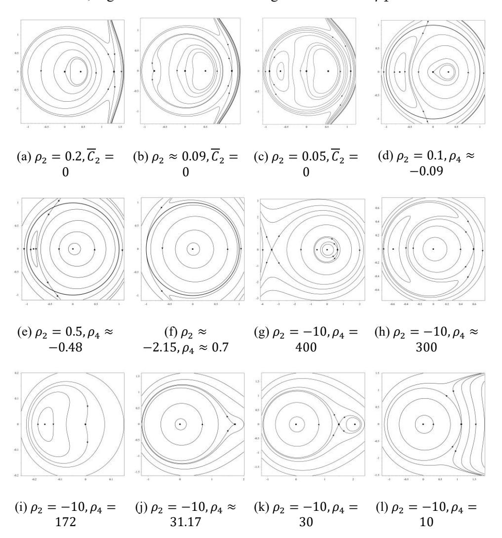
Figure 3 Some phase portraits of the system derived from the Hamiltonian (16) for ¹ = 0, ⁰ = 1. Saddle-center bifurcations occur in (a)-(c), (h)-(i), and (j)-(k). In (d)-(f), a circle as a manifold of equilibria is present. From (g) to (h), the saddle point shifts left and eventually dissapears. Similarly, from (k) to (l), the right center point shifts right before vanishing.

6 Concluding Remarks

Due to the existence of discrete symmetries in the FPU chain of a four alternating masses system, we can reduce the dimension of the system to a single degree of freedom system. This reduction enables us to provide the phase portrait in two-dimensional Cartesian coordinates. However, the normalization has to be done up to a higher degree to see interesting dynamics. One can see that analyzing the bifurcations in the case = 3 is quite challenging.

Due to the numerous symplectic transformations involved, interpreting the original system from the reduced one becomes cumbersome. However, the result in the normal form is valid qualitatively. Nevertheless, this procedure generates many interesting Hamiltonian systems that will be explored in the future. This also broadens the application of normalization beyond its common use in assessing the integrability of a system. We are currently extending this approach to the inhomogeneous chain of 3 and 4 particles to further investigate the dynamics of the system for various resonances.

There is an indication that periodic FPU chains may serve as a model for planetary interactions, since the dynamics of the reduced systems in this paper (Figure 1, 2, and 3) resemble those observed by Pousse and Alessi in [13], Huang et al. in [14], Li et al. in [15], and Dam et al. in [16]. A potential direction for future research is to relax the nearest-neighbor interaction assumption to develop a more accurate model of planetary dynamics.

Acknowledgement

This research is supported by Riset P2MI FMIPA ITB 2024.