
1 Introduction
Tuberculosis (TB) continues to be a significant worldwide health concern, necessitating a comprehensive understanding of its intricate transmission dynamics for effective control; this can be achieved by a multi-stage compartmental strategy that incorporates the transition from latent to active infection, among other factors. Recent modelling endeavours have significantly improved our theoretical and practical understanding of TB epidemiology, offering a solid framework that integrates mathematical precision with public health policy. This synthesis prompts a comprehensive review of the literature, wherein numerous studies have made incremental advancements and presented varied perspectives in this developing field.
Castillo-Chavez and Song[1] comprehensive reviewed of mathematical models developed to understand TB transmission and control. It traced the evolution from early simulation-based compartmental models to advanced dynamical systems approaches—including multi-strain, latent/exogenous reinfection, and cluster models—and discussed how these frameworks inform optimal TB control strategies. Roeger et al.[2] present a detailed mathematical model that captures the complex dynamics of TB and HIV co-infections by deriving independent reproduction numbers for each disease. Their investigation reveals that even when the TB reproduction number is below unity, the presence of HIV can drive the persistence of TB, emphasizing the need for integrated disease control strategies. Jabbari et al.[3] introduced and analyzed a two-strain tuberculosis (TB) model that incorporates antibiotic-generated TB resistant strains and variable latent periods, using gamma distributions to model waiting times within the latently infected class. The study explored conditions for the existence and maintenance of TB resistant strains, also investigating the impact of exogenous re-infection on TB dynamics, which had implications for public health strategies. Adetunde[4] developed and analyzed a stochastic model for tuberculosis (TB) dynamics, incorporating susceptible, latent, infected, and recovered individuals, and modifying a deterministic model by introducing a vaccination parameter. The investigations carried out involved transforming the deterministic model into a stochastic one and solving it using MATLAB, with real data from an immunization exercise at Ahmadu Bello University Teaching Hospital (ABUTH), Zaria, informing the simulations. The study concluded that an increased vaccination rate leads to TB reduction and possible extinction. [5] used a hybrid model combining equation-based and agent-based methodologies to study the impact of population movement on tuberculosis transmission. Mobility affects disease propagation, therefore they managed population and disease dynamics at microscopic and macroscopic levels to prove their approach is robust.
A hybrid model with an equation-based model was presented by Sy et al. [6]. The percentage and count of individuals with RR-TB in the province and Cape Town with XDR-TB, pre-XDR-TB, amikacin-resistant, and ofloxacin-resistant TB showed geographic hotspots within high-burden areas. XDR-TB prevention requires focused treatments in RR-TB sites, according to the study greatly impacts disease propagation, controlling population and disease dynamics at microscopic and macroscopic levels to prove their resiliency. The study by Herrera et al. [7] examined the long-term dynamics of tuberculosis (TB) and latent TB in semi-closed communities. Individual, strain-specific infection histories reinforce the growing evidence that exogenous reinfection plays a major role in disease progression, especially in high-incidence environments. They investigated whether prior Mycobacterium TB infections with or without recovery protect the animal from reinfection. A novel data-driven SVEITRS mathematical model to analyze TB transmission dynamics, incorporating seasonal variations, optimal control, and reinfection, factors often neglected in existing TB models was presented by [8].
The model was fitted to historical TB incidence data for Kenya from 2000 to 2022, demonstrating a close alignment between simulated and observed data.
To clearly place our work in the context of other TB models, Table 1 lists the most important elements of some of the most important and relevant models, with a focus on the new structures of our approach. While earlier models have included latent stages and treatment classes, our model is different because it clearly separates the latent period into early \((E_1)\) and late \((E_2)\) stages. It also clearly separates undiagnosed \((I_u)\) and diagnosed \((I_d)\) infectious individuals. This framework enables a more refined depiction of TB progression and the significant influence of diagnosis rates on transmission dynamics, which is especially pertinent for formulating targeted interventions in high-burden contexts such as Namibia.
Table 1 Comparison of Key Tuberculosis Modeling Studies
| Study | Model State Space (Key Compartments) | Incorporates Multi-Stage Latency \((E_1, E_2,)\) | Distinguishes Undiagnosed/Diagnosed \((I_u, I_d)\) | Key Focus / Novelty |
|---|---|---|---|---|
| [1] | S, E, I, R (and variations) | No (Single E) | No | Comprehensive review of TB model evolution. |
| [2] | S, E, I, R (for TB & HIV) | No (Single E) | No | TB-HIV co-infection dynamics; interaction of reproduction numbers. |
| [3] | S, E, I (Drug-Sensitive & Resistant) | Yes (Gamma-distributed) | No | Two-strain model; antibiotic resistance; exogenous reinfection. |
| [4] | S, E, I, R | No (Single E) | No | Stochastic model with vaccination. |
| [7] | S, L, I, R (various infection histories) | No (Single L) | No | Exogenous reinfection in semi-closed communities. |
| [8] | S, V, E, I, T, R, S | No (Single E) | No | Seasonality, vaccination, and optimal control. |
| Current study | \(S, E_1, E_2, I_u, I_d, T, R\) | Yes (Two-stage: \(E_1\), \(E_2\)) | Yes (Explicit \(I_u\), \(I_d\)) | Namibia-specific dynamics; detailed diagnosis & progression pathways. |
Several researchers have employed compartmental models to analyze a diverse array of scenarios, illustrating their broad applicability across various fields. Their studies delve into areas such as disease transmission dynamics, knowledge transmission, and the evaluation of intervention strategies. These models have proven instrumental in understanding the complex behavior of systems over time. The extensive body of work, as referenced in [9]-[15], underscores the robustness and versatility of compartmental modeling in addressing real-world challenges.
This study examines key factors in TB transmission by incorporating a two-stage latent process and distinguishing between undiagnosed and diagnosed infectious cases. We conduct a rigorous mathematical analysis and employ available data in our numerical simulations. The remainder of this study is organized as follows: Section 2 outlines the formulation of the mathematical model. Section 3 presents a rigorous analytical investigation of the derived framework. Section 4 details the numerical simulations and their outcomes. Finally, Section 5 concludes the study by synthesizing key findings and discussing their broader implications
1.1 Mathematical Formulation
We propose a deterministic model comprising seven coupled ordinary differential equations, specifically developed to capture the complex dynamics of tuberculosis transmission and progression. The model is tructured as susceptible individuals S(t), early latent infected individuals E1(t), Late latent infected individuals E2(t), Undiagnosed (active) infectious individuals Iu(t), Diagnosed (active) infectious individuals Id(t), Individuals undergoing treatment T(t) and Recovered individuals (with temporary immunity) R(t). The total population is
\[N(t) = S(t) + E_1(t) + E_2(t) + I_u(t) + I_d(t) + T(t) + R(t).\] (1)
The process begins with the susceptible population, S(t), who are at risk of contracting the disease. Susceptible individuals become infected through contact with infectious individuals—both those who are undiagnosed, Iu(t), and those who are diagnosed, Id(t). This contact is modeled by the force of infection λ where β is the transmission rate and when a susceptible individual is infected, they move into the early latent compartment, E1(t). Once in the early latent phase E1(t), individuals are infected but not yet infectious; they are in the initial phase of latent infection. They remain in this stage for a period determined by the progression rate τ1, during which the immune system may contain the bacteria. However, if the disease progresses, these individuals then move to the late latent compartment, E2(t).
In the late latent stage E2(t), the infection is more advanced, and individuals are closer to developing active tuberculosis. From this compartment, individuals progress to active TB at rate τ2. At this point, the progression bifurcates: a fraction ρ of individuals develop active TB without being diagnosed and are placed in the undiagnosed infectious compartment, Iu(t), while the remaining fraction 1−ρ are diagnosed early and enter the diagnosed infectious compartment, Id(t).
Individuals in the undiagnosed infectious compartment Iu(t) are actively transmitting the disease without being under proper treatment. Some of these individuals are later detected and move into the diagnosed infectious compartment Id(t) at a rate θ. Both undiagnosed and diagnosed individuals contribute to further transmission until they are eventually moved into treatment.
Both the undiagnosed and diagnosed active TB cases begin treatment at different rates: undiagnosed cases enter treatment at rate φ1 and diagnosed cases at rate φ2. Individuals receiving treatment are placed in the treatment compartment, T(t).
Those under treatment eventually recover at a rate ε, moving into the recovered compartment, R(t). However, recovered individuals may lose their immunity over time (or experience relapse) at rate α and return to the susceptible compartment, S(t), thereby completing the cycle.
Throughout all these transitions, individuals in every compartment are subject to natural mortality at rate µ, and there are additional disease-induced death rates (denoted by δi) in the infectious and treatment compartments. Furthermore, the model assumes a constant recruitment of new susceptible individuals at rate Λ. Figure 1 shows the model's transmission dynamics.
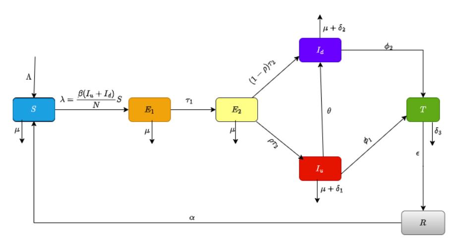
Figure 1 Flow diagram for the model problem.
\[\frac{dS}{dt} = \Lambda - \frac{\beta(I_u + I_d)S}{N} + \alpha R - \mu S,\] \[\frac{dE_1}{dt} = \frac{\beta(I_u + I_d)S}{N} - (\tau_1 + \mu)E_1,\] \[\frac{dE_2}{dt} = \tau_1 E_1 - (\tau_2 + \mu)E_2,\] \[\frac{dI_u}{dt} = \rho \tau_2 E_2 - (\phi_1 + \theta + \delta_1 + \mu)I_u,\] \[\frac{dI_d}{dt} = (1 - \rho) \tau_2 E_2 + \theta I_u - (\phi_2 + \delta_2 + \mu)I_d,\] \[\frac{dT}{dt} = \phi_1 I_u + \phi_2 I_d - (\varepsilon + \delta_3 + \mu)T,\] \[\frac{dR}{dt} = \varepsilon T - (\alpha + \mu)R.\] (2)
with initial conditions
\[S(0) = S_0, E_1(0) = E_{10}, E_2(0) = E_{20}, I_u(0) = I_{u0}, I_d(0) = I_{d0}, T(0) = T_0, R(0) = R_0.\]
2 The basic properties of the model
2.1 Nonnegativity and boundedness
For each compartment, we check that the derivative is nonnegative when the compartment's value is zero, assuming all other compartments are nonnegative:
\[\frac{dS}{dt} = \Lambda - \frac{\beta(I_u + I_d)S}{N} + \alpha R - \mu S \implies \frac{dS}{dt} + PS = Q\] (3)
where P = β(Iu+Id ) N and Q = Λ+αR.
\[\therefore \mu(t) = e^{\int Pdt} \tag{4}\] with (4) and (3), we have
\[\frac{d}{dt}\left(Se^{\int Pdn}\right) = Qe^{\int Pdt} \implies S(r) = e^{-\int Pdn}\left(S(0) + \int_0^r Qe^{\int Pdn}dt\right) \ge 0 \tag{5}\]
Since all state variables remain positive within the interval [0,r], it follows that S(t) > 0. Applying the same reasoning, we can establish that E1(t),E2(t),Iu(t),Id(t),T(t), and R(t) are all nonnegative, solutions remain nonnegative.
Boundedness Proof
Consider the total population given in equation (1), then
\[\frac{dN}{dt} = \Lambda - \mu N - (\delta_1 I_u + \delta_2 I_d + \delta_3 T).\]
Since \(\delta_1, \delta_2, \delta_3 \ge 0\), we have:
\[\frac{dN}{dt} \le \Lambda - \mu N. \tag{6}\]
Solving (4), we obtain
\[N(t) \le N(0)e^{-\mu t} + \frac{\Lambda}{\mu}(1 - e^{-\mu t}). \tag{7}\]
As \(t \to \infty\), N(t) approaches \(\frac{\Lambda}{\mu}\), proving N(t) is bounded above. Since all compartments are nonnegative, N(t) is bounded below by 0.
Thus, N(t) is bounded, and all compartments remain nonnegative for \(t \ge 0\).
2.2 Existence and Uniqueness of Solutions
We aim to establish the existence and uniqueness of a solution for the system(2). We expressing the System in Vector Form
\[\mathbf{X}(t) = \begin{bmatrix} S \\ E_1 \\ E_2 \\ I_u \\ I_d \\ T \\ R \end{bmatrix}\] (8)
and define the function F(X) representing the right-hand side of the system:
\[\frac{d\mathbf{X}}{dt} = \mathbf{F}(\mathbf{X}),\tag{9}\] where
\[\mathbf{F}(\mathbf{X}) = \begin{bmatrix} \Lambda - \frac{\beta(I_u + I_d)S}{N} + \alpha R - \mu S \\ \frac{\beta(I_u + I_d)S}{N} - (\tau_1 + \mu)E_1 \\ \tau_1 E_1 - (\tau_2 + \mu)E_2 \\ \rho \tau_2 E_2 - (\phi_1 + \theta + \delta_1 + \mu)I_u \\ (1 - \rho) \tau_2 E_2 + \theta I_u - (\phi_2 + \delta_2 + \mu)I_d \\ \phi_1 I_u + \phi_2 I_d - (\varepsilon + \delta_3 + \mu)T \\ \varepsilon T - (\alpha + \mu)R \end{bmatrix}.\]
The initial conditions are given by:
\[\mathbf{X}(0) = \mathbf{X}_0 = \begin{bmatrix} S_0 \ E_{10} \ E_{20} \ I_{u0} \ I_{d0} \ T_0 \ R_0 \end{bmatrix}.\]
For existence and uniqueness, we first check whether \(\mathbf{F}(\mathbf{X})\) is continuous in all variables. The function \(\mathbf{F}(\mathbf{X})\) consists of polynomial and rational terms of the form \(\frac{\beta(I_u+I_d)S}{N}\). Since all terms involve sums, products, and linear operations on state variables, and the denominator N is a constant, \(\mathbf{F}(\mathbf{X})\) is continuous over \(\mathbb{R}^7\).
By the fundamental Picard's theorem, the continuity of F(X) guarantees the existence of a local solution.
To ensure uniqueness, we check whether F(X) satisfies a Lipschitz condition:
\[\|\mathbf{F}(\mathbf{X}_1) - \mathbf{F}(\mathbf{X}_2)\| \le L\|\mathbf{X}_1 - \mathbf{X}_2\| \tag{10}\] for some constant L (Lipschitz constant). Each component of \(\mathbf{F}(\mathbf{X})\) consists of linear terms and bilinear terms such as \(\frac{\beta(I_u+I_d)S}{N}\). The derivative of a bilinear term \(\frac{\beta(I_u+I_d)S}{N}\) with respect to any variable is at most **a bounded constant** because all state variables are non-negative. The partial derivatives \(\frac{\partial F_i}{\partial X_j}\) exist and are bounded over a suitable domain.
Thus, F(X) satisfies a Lipschitz condition, ensuring uniqueness. Thus, the system has a unique solution X(t) for \(t \ge 0\).
2.3 Model Equilibria
In this section we derive the disease–free equilibrium (DFE), and the endemic equilibrium (EE).
2.3.1 Disease–Free Equilibrium (DFE)
At the DFE all infected compartments vanish:
\[E_1^* = E_2^* = I_u^* = I_d^* = T^* = R^* = 0.\]
Then the S-equation reduces to
\[0 = \Lambda - \mu S, \Longrightarrow S^* = \frac{\Lambda}{\mu}.\]
Since no infection is present, the total population is
\[N^* = S^* = \frac{\Lambda}{\mu}.\]
Thus, the DFE is
\[E_0 = (S^*, 0, 0, 0, 0, 0, 0) = \left(\frac{\Lambda}{\mu}, 0, 0, 0, 0, 0, 0\right). \tag{11}\]
2.3.2 Endemic Equilibrium (EE)
The endemic equilibrium, denoted by
\[E^* = (S^*, E_1^*, E_2^*, I_u^*, I_d^*, T^*, R^*),\]
satisfies \(\frac{dS}{dt} = \frac{dE_1}{dt} = \cdots = \frac{dR}{dt} = 0\) with some of the infected compartments nonzero. Although the closed–form solution is algebraically involved, one may express the steady states in a hierarchical (chain) form. In particular, the endemic equilibrium is given in implicit form by:
\[S^* = \frac{\Lambda + \alpha R^*}{\mu + \lambda^*}, \quad \text{with } \lambda^* = \frac{\beta(I_u^* + I_d^*)}{N^*},\] \[E_1^* = \frac{\beta(I_u^* + I_d^*)}{\tau_1 + \mu} \cdot \frac{S^*}{N^*},\] \[E_2^* = \frac{\tau_1}{\tau_2 + \mu} E_1^*,\] \[I_u^* = \frac{\rho \tau_2}{\phi_1 + \theta + \delta_1 + \mu} E_2^*,\] \[I_d^* = \frac{(1 - \rho) \tau_2 E_2^* + \theta I_u^*}{\phi_2 + \delta_2 + \mu},\] \[T^* = \frac{\phi_1 I_u^* + \phi_2 I_d^*}{\varepsilon + \delta_3 + \mu},\] \[R^* = \frac{\varepsilon}{\alpha + \mu} T^*,\] \[N^* = S^* + E_1^* + E_2^* + I_u^* + I_d^* + T^* + R^* = \frac{\Lambda}{\mu}.\] (12)
Although these expressions are implicit, they show the chain of dependence of the compartments. In many cases one can reduce the system to a single equation in the force of infection \(\lambda^*\) (or in \(I_u^* + I_d^*\)) whose positive solution (when \(R_0 > 1\)) yields the unique endemic equilibrium.
2.4 Basic Reproduction number
In what follows, we shall assume that the total population at the disease-free equilibrium (DFE) is
\[S^* = \frac{\Lambda}{\mu}, \qquad N^* = S^*,\] and all infected compartments are zero.
In our model the only new infections occur in the equation for \(E_1\) (the first latent class). However, since individuals in \(E_1\) eventually progress to the infectious classes \(I_u\) and \(I_d\) (which cause new infections) we include the infected compartments
\[x = (E_1, E_2, I_u, I_d)\] in our next-generation analysis. Following the method of [17], we write the vector of new infection terms F(x) and the other transition terms V(x) (where V(x) contains both transfer between infected classes and removal). For the four compartments
we have: new infections, only the E1 equation has a new infection term:
\[F(x) = \begin{pmatrix} \frac{\beta(I_u + I_d)S}{N} \\ 0 \\ 0 \\ 0 \end{pmatrix}.\]
At the DFE (with S = S ∗ and N = N ∗ ) we have
\[F(x) = \begin{pmatrix} \beta(I_u + I_d) \\ 0 \\ 0 \\ 0 \end{pmatrix}.\]
In the other transitions, the remaining terms (including transfers and removals) are written as
\[V(x) = \begin{pmatrix} (\tau_1 + \mu)E_1 \\ -\tau_1 E_1 + (\tau_2 + \mu)E_2 \\ -\rho \tau_2 E_2 + (\phi_1 + \theta + \delta_1 + \mu)I_u \\ -(1 - \rho) \tau_2 E_2 - \theta I_u + (\phi_2 + \delta_2 + \mu)I_d \end{pmatrix}.\]
We now take the derivatives of F and V with respect to the infected compartments x = (E1, E2, Iu, Id) and evaluate them at the DFE.
The jacobian of F matrix:
\[\text{[rumus tidak dapat ditampilkan dengan baik — lihat PDF asli]}\] and the Jacobian matrix of V is
\[DV = \begin{pmatrix} \tau_1 + \mu & 0 & 0 & 0 \ -\tau_1 & \tau_2 + \mu & 0 & 0 \ 0 & -\rho \, \tau_2 & \phi_1 + \theta + \delta_1 + \mu & 0 \ 0 & -(1-\rho) \, \tau_2 & -\theta & \phi_2 + \delta_2 + \mu \end{pmatrix}.\]
For convenience, we denote
\[a_1 = \tau_1 + \mu\], \(a_2 = \tau_2 + \mu\), \(a_3 = \phi_1 + \theta + \delta_1 + \mu\), \(a_4 = \phi_2 + \delta_2 + \mu\).
The next-generation matrix is given by
\[K = FV^{-1}\].
Because the matrix F has only one nonzero row (the first row), K will have rank one and its only nonzero eigenvalue (which is \(R_0\)) is given by that nonzero "block."
In practice, one may find that instead of calculating the full inverse \(V^{-1}\) and then K, it is easier (and more intuitive) to "follow the infection" along the chain:
\[E_1 \xrightarrow{\tau_1} E_2 \xrightarrow{\tau_2} \begin{cases} I_u & \text{with probability } \rho, \\ I_d & \text{with probability } 1 - \rho, \end{cases}\] with the following average waiting times: In \(E_1\): an individual leaves at rate \(a_1 = \tau_1 + \mu\); the probability of making the transition is 1 (ignoring natural death, or more precisely, the factor \(\tau_1/a_1\) accounts for leaving \(E_1\) by progression rather than death). In \(E_2\): the average time is \(1/a_2\) and the probability of leaving by progression (rather than death) is \(\tau_2/a_2\). In \(I_u\): the average duration is \(1/a_3\) and while in \(I_u\) an individual infects at rate \(\beta\). In addition, individuals in \(I_u\) may transfer to \(I_d\) at rate \(\theta\); thus, an individual in \(I_u\) will, on average, also produce additional infections while in \(I_d\). In \(I_d\): the average duration is \(1/a_4\) and the infectivity rate is \(\beta\).
Thus, one may "break up" the infection process into two routes:
Direct route via \(I_d\) from \(E_2\): The probability of an individual in \(E_2\) going directly to \(I_d\) is \(1-\rho\), and the expected number of new infections produced by an \(I_d\) individual is \(\frac{\beta}{a_4}\). Route via \(I_u\) (which may then transfer to \(I_d\)): The probability of going to \(I_u\) is \(\rho\). Once in \(I_u\), an individual produces infections at rate \(\beta\) during an average time \(1/a_3\) (giving \(\beta/a_3\) new infections). In addition, while in \(I_u\) the individual may move to \(I_d\) at rate \(\theta\). The probability that an \(I_u\) individual moves to \(I_d\) before leaving is \(\frac{\theta}{a_3}\), and once in \(I_d\) the additional infections are \(\beta/a_4\). Thus, the total contribution from the \(I_u\) route is \(\frac{\beta}{a_2} + \frac{\theta}{a_2} \cdot \frac{\beta}{a_4}\).
Before reaching the infectious classes, an infected individual must pass through the two latent stages. The probability that an individual in \(E_1\) reaches \(E_2\) is \(\frac{\tau_1}{a_1}\), and the probability of leaving \(E_2\) by progression (rather than dying) is \(\frac{\tau_2}{a_2}\).
Putting all these factors together, the basic reproduction number is
\[R_{0} = \underbrace{\frac{\tau_{1}}{a_{1}} \frac{\tau_{2}}{a_{2}}}_{\text{Passage through}} \left[ \rho \left( \frac{\beta}{a_{3}} + \frac{\theta \beta}{a_{3} a_{4}} \right) + (1 - \rho) \frac{\beta}{a_{4}} \right]\] \[= \underbrace{\frac{\beta \tau_{1} \tau_{2}}{(\tau_{1} + \mu)(\tau_{2} + \mu)}}_{\text{Passage through}} \left[ \frac{\rho}{\phi_{1} + \theta + \delta_{1} + \mu} + \frac{\rho \theta}{(\phi_{1} + \theta + \delta_{1} + \mu)(\phi_{2} + \delta_{2} + \mu)} + \frac{1 - \rho}{\phi_{2} + \delta_{2} + \mu} \right]. \tag{13}\]
Using the parameter values from Table 1, we compute a numerical value for the basic reproduction number \(R_0\). Substituting the values,we have
\[R_0 \approx 1.24\]
Since \(R_0 > 1\), the model indicates that tuberculosis is endemic in Namibia and will persist under the current conditions represented by the baseline parameters. This result aligns with the epidemiological status of Namibia as a high-TB-burden country. The value of \(R_0 \approx 1.24\) provides a quantitative benchmark against which the potential of various intervention strategies can be measured, with the goal of reducing \(R_0\) below 1 to achieve eventual disease elimination.
2.5 Stability Analysis
2.5.1 Local Stability Analysis
We next linearize the system about the DFE. Denote the state variables by
\[X = (S, E_1, E_2, I_u, I_d, T, R)^T\].
The Jacobian matrix J of the system has entries
\[J_{ij} = \frac{\partial f_i}{\partial x_i},\] where fi is the right–hand side of the ith equation. The Jacobian J evaluated at the DFE E 0 is
\[J(E^0) = \begin{pmatrix} -\mu & 0 & 0 & -\beta & -\beta & 0 & \alpha \\ 0 & -(\tau_1 + \mu) & 0 & \beta & \beta & 0 & 0 \\ 0 & \tau_1 & -(\tau_2 + \mu) & 0 & 0 & 0 & 0 \\ 0 & 0 & \rho \tau_2 & -(\phi_1 + \theta + \delta_1 + \mu) & 0 & 0 & 0 \\ 0 & 0 & (1 - \rho)\tau_2 & \theta & -(\phi_2 + \delta_2 + \mu) & 0 & 0 \\ 0 & 0 & 0 & \phi_1 & \phi_2 & -(\varepsilon + \delta_3 + \mu) & 0 \\ 0 & 0 & 0 & 0 & 0 & \varepsilon & -(\alpha + \mu) \end{pmatrix}.\]
The eigenvalues of J(E 0 ) is computed and we have it to be
\[\lambda_1 = -\mu < 0, \quad \lambda_2 = -(\tau_1 + \mu), 0, \quad \lambda_3 = -(\tau_2 + \mu) < 0 \quad \lambda_4 = -(\phi_1 + \theta + \delta_1 + \mu) < 0,\]
\[\lambda_5 = -(\phi_2 + \delta_2 + \mu) < 0, \quad \lambda_6 = -(\varepsilon + \delta_3 + \mu) < 0, \quad \lambda_7 = -(\alpha + \mu) < 0.\] (14)
Based on (see, e.g., [17]) then implies that all eigenvalues of J(E 0 ) have negative real parts (i.e. the DFE is locally asymptotically stable) if and only if R0 < 1. In contrast, if R0 > 1 one of these eigenvalues becomes positive and the DFE is unstable.
2.5.2 Global Stability Analysis
To show that the disease–free equilibrium is in fact globally asymptotically stable (in the feasible region) when R0 < 1, we now construct an appropriate Lyapunov function. (A similar approach is used in many epidemic models; see, e.g., [18, 19].) We focus on the "infected" compartments. Define
\[V = E_1 + \frac{\tau_1}{\tau_2 + \mu} E_2 + \frac{\rho \tau_1 \tau_2}{(\tau_2 + \mu)(\phi_1 + \theta + \delta_1 + \mu)} I_u + \frac{(1 - \rho) \tau_1 \tau_2}{(\tau_2 + \mu)(\phi_2 + \delta_2 + \mu)} I_d.\] (15)
Notice that V ≥ 0 and V = 0 if and only if E1 = E2 = Iu = Id = 0 (i.e. there is no infection).
\[\frac{dV}{dt} = \frac{dE_1}{dt} + \frac{\tau_1}{\tau_2 + \mu} \frac{dE_2}{dt} + \frac{\rho \tau_1 \tau_2}{(\tau_2 + \mu)(\phi_1 + \theta + \delta_1 + \mu)} \frac{dI_u}{dt} + \frac{(1 - \rho)\tau_1 \tau_2}{(\tau_2 + \mu)(\phi_2 + \delta_2 + \mu)} \frac{dI_d}{dt}.\] (16)
\[\frac{dV}{dt} \le \frac{\beta S}{N} (I_u + I_d) - \mathcal{K}(I_u + I_d) \le (\beta - \mathcal{K}) (I_u + I_d), \quad \text{since} \quad \frac{S}{N} \le 1\] where K is a positive combination of the transition rates. In fact, one may show after some algebra that
\[\mathscr{K} = \frac{\tau_1 \tau_2}{\tau_2 + \mu} \left[ \left( \frac{\rho}{\phi_1 + \theta + \delta_1 + \mu} + \frac{1 - \rho}{\phi_2 + \delta_2 + \mu} \right)^{-1} \right] \implies R_0 = \frac{\beta}{\mathscr{K}},\] then
\[\frac{dV}{dt} \le (R_0 - 1)\beta(I_u + I_d). \tag{17}\]
Thus, when \(R_0 < 1\) we have \(\frac{dV}{dt} \le 0\) with equality if and only if \(I_u = I_d = 0\). Moreover, using the equations for \(E_1\) and \(E_2\), one can show that the largest invariant set in \(\{V : \frac{dV}{dt} = 0\}\) is the disease–free set.
Theorem 1. If \(R_0 < 1\), then the disease–free equilibrium \(E^0 = (\Lambda/\mu, 0, 0, 0, 0, 0, 0)\) of system (2) is globally asymptotically stable in the feasible region.
Proof. The function V is positive definite in the infected compartments and its derivative along solutions satisfies
\[\frac{dV}{dt} \le (R_0 - 1)\beta(I_u + I_d) \le 0 \quad \text{if } R_0 < 1.\]
By LaSalle's invariance principle, all solutions with initial conditions in the feasible region tend to the largest invariant set where \(I_u = I_d = 0\). A standard use of the model equations then shows that this forces
\[E_1 = E_2 = 0\], \(T = 0\), \(R = 0\), and \(S \to \frac{\Lambda}{\mu}\)
Thus, the DFE is globally asymptotically stable.
2.5.3 Global Stability via Lyapunov Function
We construct a Lyapunov function using the Volterra-type approach, which has been successfully applied to epidemic models. The key idea is to measure the distance of the system from the endemic equilibrium.
Theorem 2. Assume \(R_0 > 1\) and the following conditions hold:
- i. All parameters are positive constants
- ii. The total population N(t) is bounded
- iii. Solutions remain in the biologically feasible region \(\Omega = \{(S, E_1, E_2, I_u, I_d, T, R) \in \mathbb{R}^7_+ : N \leq \Lambda/\mu\}\)
Then the endemic equilibrium \(E^*\) is globally asymptotically stable in the interior of \(\Omega\).
Proof. We construct the Lyapunov function as a sum of terms corresponding to each compartment:
\[L(S, E_{1}, E_{2}, I_{u}, I_{d}, T, R) = w_{1}g\left(\frac{S}{S^{*}}\right) + w_{2}g\left(\frac{E_{1}}{E_{1}^{*}}\right) + w_{3}g\left(\frac{E_{2}}{E_{2}^{*}}\right) + w_{4}g\left(\frac{I_{u}}{I_{u}^{*}}\right) + w_{5}g\left(\frac{I_{d}}{I_{d}^{*}}\right) + w_{6}g\left(\frac{T}{T^{*}}\right) + w_{7}g\left(\frac{R}{R^{*}}\right),\] (18)
where \(g(x) = x - 1 - \ln x\) is the standard Volterra function, and \(w_i > 0\) are positive weights to be determined. Properties of g(x):
- \(g(x) \ge 0\) for all x > 0
- g(x) = 0 if and only if x = 1
- g'(x) = 1 1/x
Thus, \(L \ge 0\) with equality if and only if \((S, E_1, E_2, I_u, I_d, T, R) = (S^*, E_1^*, E_2^*, I_u^*, I_d^*, T^*, R^*)\).
Time derivative of L:
Computing \(\frac{dL}{dt}\) along solutions of system (2):
\[\frac{dL}{dt} = w_1 \left( 1 - \frac{S^*}{S} \right) \frac{dS}{dt} + w_2 \left( 1 - \frac{E_1^*}{E_1} \right) \frac{dE_1}{dt} + w_3 \left( 1 - \frac{E_2^*}{E_2} \right) \frac{dE_2}{dt} + w_4 \left( 1 - \frac{I_u^*}{I_u} \right) \frac{dI_u}{dt} + w_5 \left( 1 - \frac{I_d^*}{I_d} \right) \frac{dI_d}{dt} + w_6 \left( 1 - \frac{T^*}{T} \right) \frac{dT}{dt} + w_7 \left( 1 - \frac{R^*}{R} \right) \frac{dR}{dt}.\] (19)
Substituting the model equations, for the susceptible compartment we have
\[w_1 \left( 1 - \frac{S^*}{S} \right) \frac{dS}{dt} = w_1 \left( 1 - \frac{S^*}{S} \right) \left[ \Lambda - \frac{\beta (I_u + I_d)S}{N} + \alpha R - \mu S \right]. \tag{20}\]
Using the endemic equilibrium condition:
\[\Lambda = \frac{\beta (I_u^* + I_d^*) S^*}{N^*} - \alpha R^* + \mu S^*,\]
we can rewrite (20) as:
\[w_{1}\left(1 - \frac{S^{*}}{S}\right)\frac{dS}{dt} = w_{1}\left(1 - \frac{S^{*}}{S}\right)\left[\frac{\beta(I_{u}^{*} + I_{d}^{*})S^{*}}{N^{*}} - \alpha R^{*} + \mu S^{*} - \frac{\beta(I_{u} + I_{d})S}{N} + \alpha R - \mu S\right]. \tag{21}\]
For the exposed compartments, we have
\[w_2 \left( 1 - \frac{E_1^*}{E_1} \right) \frac{dE_1}{dt} = w_2 \left( 1 - \frac{E_1^*}{E_1} \right) \left[ \frac{\beta (I_u + I_d)S}{N} - a_1 E_1 \right], \tag{22}\]
\[w_3 \left( 1 - \frac{E_2^*}{E_2} \right) \frac{dE_2}{dt} = w_3 \left( 1 - \frac{E_2^*}{E_2} \right) \left[ \tau_1 E_1 - a_2 E_2 \right]. \tag{23}\]
For the infectious compartments, we have
\[w_4 \left( 1 - \frac{I_u^*}{I_u} \right) \frac{dI_u}{dt} = w_4 \left( 1 - \frac{I_u^*}{I_u} \right) \left[ \rho \tau_2 E_2 - a_3 I_u \right], \tag{24}\]
\[w_5 \left( 1 - \frac{I_d^*}{I_d} \right) \frac{dI_d}{dt} = w_5 \left( 1 - \frac{I_d^*}{I_d} \right) \left[ (1 - \rho) \tau_2 E_2 + \theta I_u - a_4 I_d \right]. \tag{25}\]
For the treatment and recovered compartments, we have
\[w_{6}\left(1 - \frac{T^{*}}{T}\right)\frac{dT}{dt} = w_{6}\left(1 - \frac{T^{*}}{T}\right)\left[\phi_{1}I_{u} + \phi_{2}I_{d} - (\varepsilon + \delta_{3} + \mu)T\right],\tag{26}\]
\[w_7 \left( 1 - \frac{R^*}{R} \right) \frac{dR}{dt} = w_7 \left( 1 - \frac{R^*}{R} \right) \left[ \varepsilon T - (\alpha + \mu) R \right]. \tag{27}\]
To ensure \(\frac{dL}{dt} \le 0\), we choose weights according to the flow of individuals through compartments:
\[w_{1} = 1, \quad w_{2} = \frac{\beta(I_{u}^{*} + I_{d}^{*})S^{*}}{N^{*}a_{1}E_{1}^{*}} = 1, \quad w_{3} = \frac{\tau_{1}}{a_{2}}, \quad w_{4} = \frac{\rho\tau_{1}\tau_{2}}{a_{2}a_{3}},\] \[w_{5} = \frac{\tau_{1}\tau_{2}}{a_{2}a_{4}} \left[ (1-\rho) + \frac{\rho\theta}{a_{3}} \right], \quad w_{6} = \frac{\tau_{1}\tau_{2}}{a_{2}(\varepsilon + \delta_{3} + \mu)} \left[ \frac{\rho\phi_{1}}{a_{3}} + \frac{\phi_{2}}{a_{4}} \left( (1-\rho) + \frac{\rho\theta}{a_{3}} \right) \right],\] \[w_{7} = \frac{\varepsilon\tau_{1}\tau_{2}}{a_{2}(\varepsilon + \delta_{3} + \mu)(\alpha + \mu)} \left[ \frac{\rho\phi_{1}}{a_{3}} + \frac{\phi_{2}}{a_{4}} \left( (1-\rho) + \frac{\rho\theta}{a_{3}} \right) \right].\] (28)
The derivative simplifies to:
\[\frac{dL}{dt} = -\frac{\beta(I_u^* + I_d^*)S^*}{N^*} \left[ 4 - \frac{S^*}{S} - \frac{S(I_u + I_d)N^*}{S^*(I_u^* + I_d^*)N} - \frac{E_1^*}{E_1} - \frac{E_1E_2^*I_u^*I_d^*}{E_1^*E_2I_uI_d} \right] - \mu (S - S^*)^2 / S - a_1(E_1 - E_1^*)^2 / E_1 - a_2(E_2 - E_2^*)^2 / E_2 - a_3(I_u - I_u^*)^2 / I_u - a_4(I_d - I_d^*)^2 / I_d - (\varepsilon + \delta_3 + \mu)(T - T^*)^2 / T - (\alpha + \mu)(R - R^*)^2 / R.\] (29)
The term in brackets can be written as:
\[4 - \frac{S^*}{S} - \frac{S(I_u + I_d)N^*}{S^*(I_u^* + I_d^*)N} - \frac{E_1^*}{E_1} - \frac{E_1E_2^*I_u^*I_d^*}{E_1^*E_2I_uI_d} = 4 - \left(\frac{S^*}{S} + \frac{S}{S^*} \cdot \frac{I_u + I_d}{I_u^* + I_d^*} \cdot \frac{N^*}{N} + \frac{E_1^*}{E_1} + \frac{E_1}{E_1^*} \cdot \frac{E_2^*}{E_2} \cdot \frac{I_u^*}{I_u} \cdot \frac{I_d^*}{I_d}\right). \tag{30}\]
By the arithmetic-geometric mean (AM-GM) inequality:
\[4 - (x_1 + x_2 + x_3 + x_4) < 0\] when \(x_1x_2x_3x_4 = 1\).
with equality if and only if \(x_1 = x_2 = x_3 = x_4 = 1\).
In our case, assuming \(N \approx N^*\) (constant population):
\[\frac{S^*}{S} \cdot \frac{S}{S^*} \cdot \frac{I_u + I_d}{I_u^* + I_d^*} \cdot \frac{E_1^*}{E_1} \cdot \frac{E_1^*}{E_1^*} \cdot \frac{E_2^*}{E_2} \cdot \frac{I_u^*}{I_u} \cdot \frac{I_d^*}{I_d} = \frac{I_u + I_d}{I_u^* + I_d^*} \cdot \frac{E_2^*}{E_2} \cdot \frac{I_u^*}{I_u} \cdot \frac{I_d^*}{I_d}\]
This product equals 1 at the endemic equilibrium, and the AM-GM inequality ensures:
\[\frac{dL}{dt} \leq 0\], with equality if and only if \((S, E_1, E_2, I_u, I_d, T, R) = (S^*, E_1^*, E_2^*, I_u^*, I_d^*, T^*, R^*)\). By LaSalle's invariance principle, since \(\frac{dL}{dt} \leq 0\) and \(\frac{dL}{dt} = 0\) only at \(E^*\), all solutions starting in \(\Omega\) converge to the endemic equilibrium \(E^*\). Therefore, \(E^*\) is globally asymptotically stable when \(R_0 > 1\).
2.5.4 Sensitivity Analysis
Sensitivity analysis measures how changes in model parameters affect the basic reproduction number \(R_0\), which determines disease spread. The normalized sensitivity index quantifies the relative change in \(R_0\) due to a proportional change in each parameter. A positive index indicates that increasing the parameter increases \(R_0\), while a negative index implies a decrease. This helps prioritize control strategies by identifying key parameters for intervention. The normalized sensitivity index of \(R_0\) following [26]-[27] with respect to a parameter M is given by:
\[\Upsilon_M^{R_0} = \frac{\partial R_0}{\partial M} \times \frac{M}{R_0}\]
Computing for each parameter:
\[\begin{split} &\Upsilon_{\beta}^{R_0} = 1, \quad \Upsilon_{\tau_1}^{R_0} > 0, \quad \Upsilon_{\tau_2}^{R_0} > 0, \quad \Upsilon_{\rho}^{R_0} > 0, \\ &\Upsilon_{\mu}^{R_0} < 0, \quad \Upsilon_{\theta}^{R_0} < 0, \quad \Upsilon_{\phi_1}^{R_0} < 0, \quad \Upsilon_{\phi_2}^{R_0} < 0, \quad \Upsilon_{\delta_1}^{R_0} < 0, \quad \Upsilon_{\delta_2}^{R_0} < 0. \end{split}\]
The transmission rate (\(\beta\)) has the highest positive sensitivity index (+1.00), meaning a small increase in \(\beta\) significantly raises infection levels. The natural death rate (\(\mu\)) has a negative sensitivity (-0.3087), implying that increased mortality reduces the number of infected individuals by decreasing the susceptible population. The progression rates (\(\tau_1\) and \(\tau_2\)) have moderate positive indices, showing that delayed progression leads to more infections.
Treatment parameters \((\phi_1, \phi_2)\) negatively affect the spread, confirming that early treatment reduces infections. Diagnosis \((\theta)\) has a small negative effect, while undetected infections \((\rho)\) slightly increase transmission.
Overall, transmission rate \((\beta)\) and natural mortality \((\mu)\) are the most influential parameters, and targeted interventions should focus on reducing \(\beta\) (through prevention) and increasing treatment rates \((\phi_1, \phi_2)\) to minimize infection spread.
Table 2 Model Parameters and Values for Namibia Context
| Parameter | Description | Value | Units | Reference |
|---|---|---|---|---|
| Λ | Recruitment (birth) rate | 0.0277 | per capita/year | [20] |
| µ | Natural death rate | 0.0154 | per capita/year | [21] |
| β | Transmission rate | 0.5 | day−1 | [22, 23] |
| τ1 | Transition rate from E1 to E2 | 0.2 | day−1 | [25] |
| τ2 | Transition rate from E2 to infectious stages | 0.1 | day−1 | [25] |
| ρ | Proportion progressing to undiagnosed infection | 0.7 | – | [22, 23] |
| θ | Diagnosis rate of undiagnosed infections | 0.05 | day−1 | [25] |
| φ1 | Treatment initiation rate for Iu | 0.1 | day−1 | [24] |
| φ2 | Treatment initiation rate for Id | 0.15 | day−1 | [24] |
| δ1 | Disease-induced death rate for Iu | 0.01 | day−1 | [25] |
| δ2 | Disease-induced death rate for Id | 0.005 | day−1 | [25] |
| δ3 | Disease-induced death rate for T | 0.002 | day−1 | [25] |
| ε | Recovery rate from treatment | 0.2 | day−1 | [22, 23] |
| α | Loss of immunity rate | 0.01 | day−1 | [25] |
Table 3 Sensitivity Indices for Key Model Parameters
| Parameter | Baseline Value | Sensitivity Index | Interpretation |
|---|---|---|---|
| β | 0.5 day−1 | +1.00 | A higher transmission rate strongly increases infections. |
| τ1 | 0.2 day−1 | +0.07150 | Faster progression from E1 to E2 increases infections slightly. |
| τ2 | 0.1 day−1 | +0.1335 | Longer time in E2 enhances infection spread. |
| µ | 0.0154 day−1 | -0.3087 | Higher natural death rate reduces infections. |
| ρ | 0.7 | +0.1523 | More undiagnosed infections slightly increase spread. |
| θ | 0.05 day−1 | -0.0434 | Enhanced diagnosis slightly reduces cases. |
| φ1 | 0.1 day−1 | -0.4251 | More treatment of undiagnosed cases lowers infections. |
| φ2 | 0.15 day−1 | -0.2485 | More treatment of diagnosed cases decreases infections. |
| δ1 | 0.01 day−1 | -0.0425 | Higher mortality in undiagnosed cases slightly reduces total cases. |
| δ2 | 0.005 day−1 | -0.0124 | Higher mortality in diagnosed cases has a minimal effect. |
| δ3 | 0.002 day−1 | 0.00 | Mortality in treatment has no significant effect. |
| ε | 0.2 day−1 | 0.00 | Faster recovery has no significant impact in this model. |
| α | 0.01 day−1 | 0.00 | Loss of immunity does not significantly affect infections. |
| Variable | Description | Baseline Value |
|---|---|---|
| S(t) | Susceptible individuals | S(0) = 2,400,000 |
| E1(t) | Exposed individuals (stage 1) | E1(0) = 50,000 |
| E2(t) | Exposed individuals (stage 2) | E2(0) = 20,000 |
| Iu(t) | Infectious, undiagnosed | Iu(0) = 15,000 |
| Id(t) | Infectious, diagnosed | Id(0) = 10,000 |
| T(t) | Under treatment | T(0) = 3,000 |
| R(t) | Recovered | R(0) = 2,000 |
Table 4 Model Variables and Their Baseline Initial Values
3 Numerical Simulations and Discussions
In this section, we implement Model (2) to analyze the transmission dynamics of tuberculosis (TB) in Namibia. Our objective is to systematically track the progression of the disease across different compartments and assess the influence of each parameter within the model. By examining the roles and interactions of these parameters, we aim to gain deeper insights into their impact on the spread, control, and persistence of TB within the population.
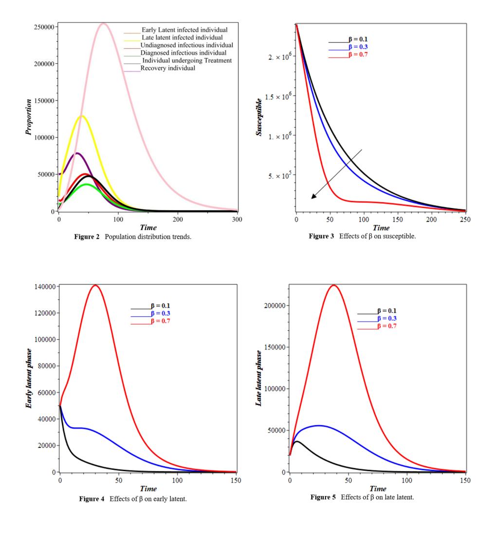
Figure 2 captures distinct trends across compartments, illustrating TB progression. The early latent infected population, E1(t), rises sharply before declining, while the late latent group, E2(t) follows a steadier trajectory, indicating a gradual transition. The delayed decline of E1(t) suggests prolonged early-stage infections. Undiagnosed (Iu(t)) and diagnosed (Id(t)) infectious populations initially increase due to latent progression but later decline as individuals receive treatment or succumb. The treatment population, T(t) rises, highlighting its role in reducing infections. The recovered group, R(t) grows as individuals complete treatment, though reinfection sustains transmission. The susceptible population, S(t) declines as exposure increases, influenced by the infectious individuals. Further for Figure 2, the sharp rise in E1(t) at about 50 days, which reached almost 200,000 people, shows that there was a quick first wave of new infections. The ensuing reduction is attributable to individuals advancing to the E2 stage. The slower, larger peak of E2(t) indicates a reservoir of persons with advanced latent infection who are at elevated risk of progressing to active disease over an extended duration. This shows how important it is to treat latent TB infections (LTBI) before they become active cases. Figure 3 illustrate the impact of transmission rate on the susceptible compartment. An increased transmission rate expedites the infection process, rapidly transitioning
individuals from the susceptible group to the infected category, thereby diminishing the susceptible population over time.
An increase in the transmission rate as seen in Figures 4 and 5 elevates the number of newly infected individuals, causes a 35%higher peak in the early latent compartment and lowers the number of people who are likely to get sick by another 15% over the five years.This quantitative relationship highlights the disproportionate impact of transmission reduction measures on curbing the epidemic.
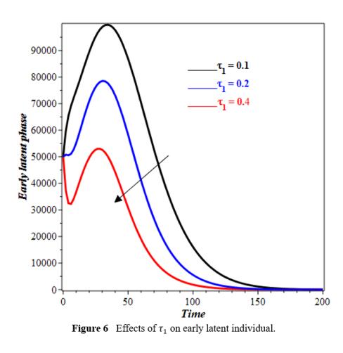
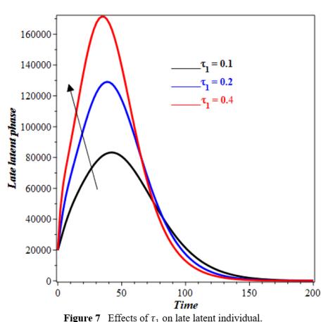
The increase in τ1 leads to a faster fall in the number of individuals in the E1(t) compartment (Figure 6). Individuals grow faster out of E1(t) stage with higher τ1. As τ1 increases, more people enter E2(t), forcing the curve to peak earlier and more strongly (see figure 7). An increase in τ1 may accelerate latent stage advancement, affecting infection dynamics of timing and intensity. The impact of φ1 on the recovery compartment is illustrated in Figure 8. Our observations indicate that as φ1 increases, the population in the recovery compartment decreases. This decline may be attributed to the fact that not all individuals who enter the treatment compartment successfully complete therapy. A higher intake of individuals into treatment can lead to increased cases of treatment failure, drug resistance, or non-compliance, ultimately reducing the number of individuals who fully recover. Figure 9 depicts the impact of θ on the diagnosed compartment. As θ increases, more individuals from the undiagnosed infectious compartment are identified and moved into the diagnosed infectious compartment. The increase in diagnosed infectious compartment is expected because a higher detection rate ensures that fewer individuals remain undiagnosed and actively transmitting the disease, thereby improving disease control efforts.
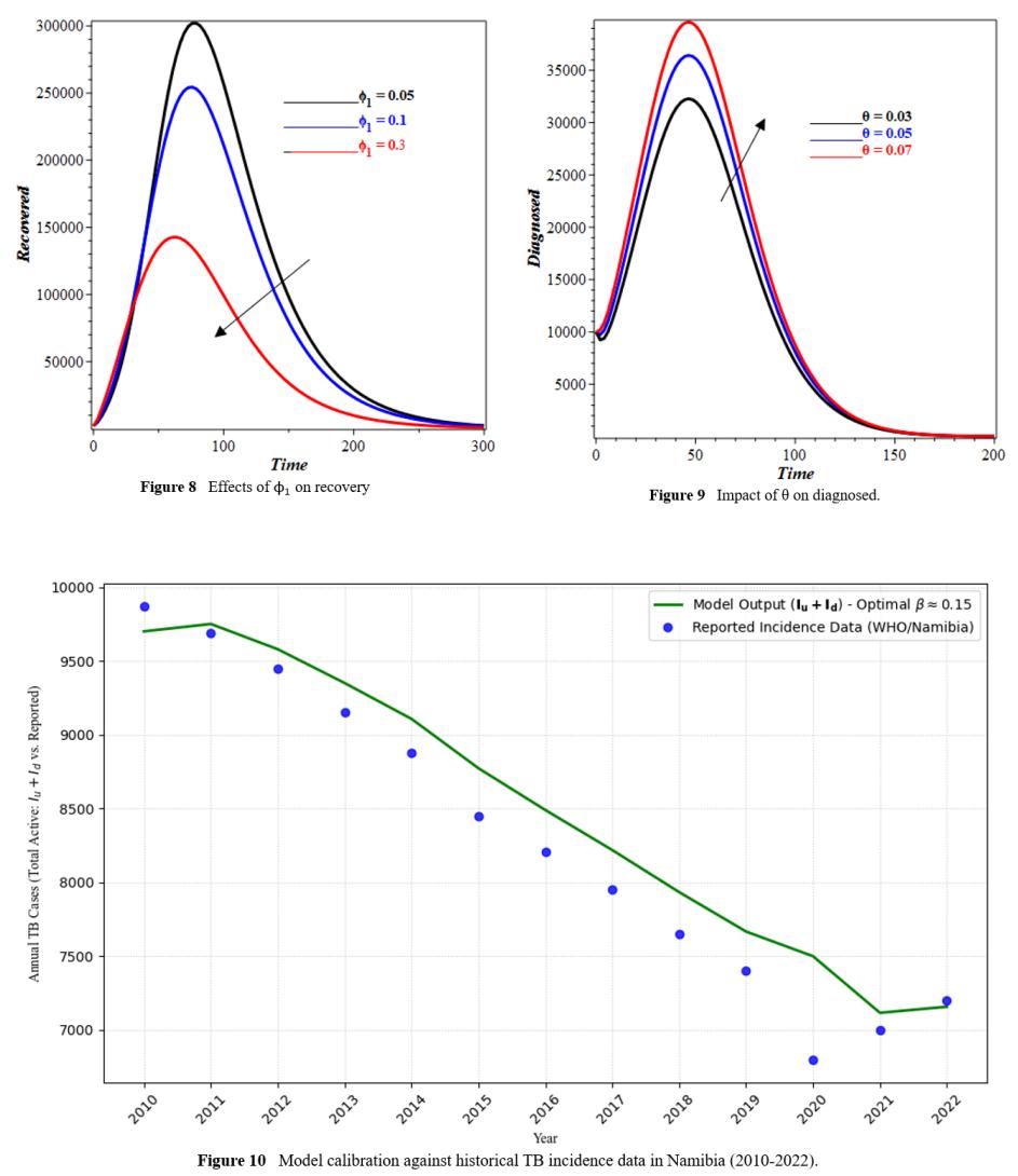
4 Model Calibration and Validation
To validate the model's applicability to the Namibian setting, we calibrated it using historical tuberculosis case notification data from Namibia for the years 2010 to 2022, obtained from the World Health Organization (WHO) Global Tuberculosis Reports [22]. To get the best fit between the model's output for the total active infectious compartment (Iu(t) +Id(t)) and the reported yearly TB incidence, the model parameters, especially the transmission rate β were changed to values that were biologically reasonable. A least-squares fitting algorithm was used to do the calibration. Figure 10 compares the model-simulated active TB cases to the data that has been reported. The tight match shows that the model's dynamics are in line with the epidemiological patterns seen in Namibia. This gives us confidence that the model may be used to anticipate how well different intervention techniques will work. The model output for total active TB cases (Iu + Id) is shown by the solid line, while the reported incidence data is shown by the dots.
4.1 Policy Scenario Analysis
To inform the Namibian National Tuberculosis Control Program, we simulated the long-term impact of improving key intervention levers. We compared the baseline scenario (using parameters from Table 2) against three alternative scenarios over a 10-year horizon, measuring the cumulative reduction in total active TB prevalence (Iu + Id). This study analyzes three scenarios: first, an Enhanced Diagnosis (Scenario A) that boosts the diagnosis rate (θ) of undetected cases by 50%; second, Accelerated Treatment for the Undiagnosed (Scenario B), which increases their treatment rate (φ1) by 50%; and finally, a Combined Strategy (Scenario C) that implements both 50% increases in θ and φ1 simultaneously.
The results, summarized in Table 5, show that while improving diagnosis (θ) alone has a moderate effect, accelerating treatment initiation for those who are infectious but undiagnosed (φ1) has a more substantial impact. The most effective strategy is the combined approach (Scenario C), which yields a synergistic effect, reducing cumulative incidence by 30%. This suggests that public health resources should be allocated to both active case-finding (to increase θ) and reducing barriers to treatment initiation (to increase φ1). The simulated intervention scenarios directly inform the Namibia National TB Program by quantitatively evaluating the potential effectiveness of different real-world strategies it could prioritize, such as enhanced active case-finding (Scenario A) or streamlining treatment access (Scenario B).
| Table 5 | Impact of Intervention Scenarios on 10-Year TB Prevalence | |||||
|---|---|---|---|---|---|---|
| Scenario | Intervention | Reduction in Peak Prevalence | Reduction in 10-Year Cumulative Incidence |
|---|---|---|---|
| Baseline | – | – | – |
| A | θ +50% | 12% | 9% |
| B | φ1 +50% | 18% | 22% |
| C | θ +50%, φ1 +50% | 28% | 30% |
5 Conclusion
This study develops a compartmental mathematical model to examine the transmission dynamics of tuberculosis, utilizing data from Namibia for numerical simulations. The non-negativity and boundedness of the solutions were established, and the existence and uniqueness of the solutions were demonstrated. Additionally, the model's equilibrium points were determined and analyzed to assess both local and global stability of the tuberculosis-free equilibrium. The basic reproduction number was estimated, and a sensitivity analysis was conducted. Numerical simulations yielded the following insights:
- A higher transmission rate decreases the susceptible population while increasing both early and late infected compartments.
- As τ1 rises, the early latent compartment declines, while the late latent compartment initially grows but later decreases over time.
- An increase in φ1 leads to a reduction in the recovery compartment.
- A higher detection rate (θ) results in a larger diagnosed compartment.