
1 Introduction
Poverty is widely acknowledged to have several dimensions, which means that persons living in poverty usually face multiple obstacles at the same time [1]. Poverty is something that society creates knowingly or unknowingly. Despite technological and knowledge advancements, poverty remains a global issue.
Although there exists a national-level Multidimensional Poverty Index (MPI) that is constructed using, health, education, and standard of living, it is vital to
1 1 Selected paper from International Conference on Computational and Mathematical Modelling (ICCMM) 2025 in Sri Lanka
consider the changing nature of societal challenges to capture the reality of poverty [2,3].
It has been pointed out that extreme weather conditions and changes in climate have been increasing over time. Record-breaking heat waves on land and in the ocean, heavy rains, severe floods, prolonged droughts, extreme wildfires, and widespread flooding during hurricanes are all becoming more frequent and more intense [4]. These are serious issues threatening human well-being and living standards.
Since all of the considered factors are naturally uncertain, a fuzzy modeling approach should be considered to measure poverty levels among households. In this study, we go beyond the traditional poverty measurement, which being solely focused on income or expenditure is insufficient to capture the true reality of poverty. Therefore, this study adopted a multidimensional poverty concept, allowing for the assessment of deprivation across multiple domains, including education, health, and standard of living.
The existing MPI captured by the Alkire Foster (AF) method considers three dimensions and ten sub-factors [5]. The combination of the headcount ratio, which represents the population proportion that lives below the poverty threshold, and the intensity of poverty produces the MPI, which provides insight into how many households are multidimensionally poor [6]. However, it is critical to identify who is the poorest among them and how to improve their living conditions.
This study sought to identify households living in poverty and classify poverty levels within those households, particularly households that may be suffering from chronic poverty. This enables the option of identifying of the poorest among the poor. After determining the poverty levels, this study aimed to identify the most significant factors that can reduce poverty among these households, thereby highlighting the dimensions that should receive greater attention. Additionally, it is crucial to examine how each factor influences household poverty, whether positively or negatively. Ultimately, the study provides policy recommendations to guide resource allocation and subsidy distribution towards the most vulnerable sectors.
2 Methodology
To classify poverty within households under the multidimensional framework, this study employed fuzzy rule-based systems and Buckley's Fuzzy Analytic Hierarchy Process (FAHP). The first step of the methodology is defining the factors that influence individuals' deprivation profiles. Figure 1 depicts the subfactors identified within the framework of each dimension. Given that many of these sub-factors are qualitative and expressed through linguistic terms, we opted for fuzzy modeling to handle both numerical and linguistic variables effectively. fuzzy set theory and fuzzy rule-based systems were used to develop the model, as they are well-suited for addressing the inherent uncertainty and imprecision in the data [7].
First, we created five different linguistic scales for the dimensions Education, Health, and Standard of Living by considering income level, education level, housing, number of dependents, environmental vulnerability, and fuzzy poverty level, designated as I, E, Hs, N, Ev, and PL, respectively. In this framework, the variables, I, E, Hs, N, Ev are considered linguistic inputs, while PL is defined as the linguistic output variable. It is important to note that the Ev factor varies significantly from country to country. It depends on the type and severity of extreme weather that can occur in that particular country and the accessibility of the data for relevant events. The developed model may be applied to developing countries also if those countries have the required survey data; usually the necessary data can be found in a country's Department of Census and Statistics (DCS), Bureau of Statistics, or Census institutions.
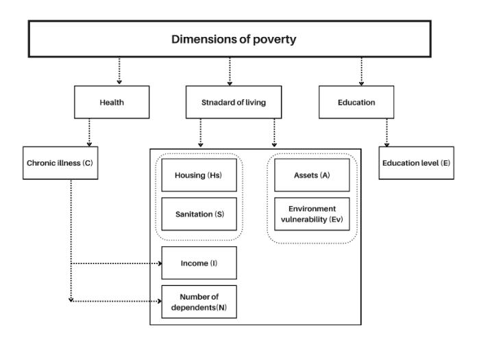
Figure 1 Dimensions (main factors) and sub-factors of multidimensional poverty.
The linguistic variables are modeled as follows:
\[I = \{I_1, I_2, I_3\}\] = \(\{L, M, H\}\),
\(E = \{E_1, E_2, E_3\}\) = \(\{L, M, H\}\),
\[HS = \{HS_1, HS_2, HS_3\} = \{L, M, H\},\\] \[N = \{N_1, N_2, N_3\} = \{L, M, H\},\\] \[Ev = \{Ev_1, Ev_2, Ev_3\} = \{L, M, H\},\\] \[PL = \{PL_1, PL_2, PL_3\} = \{P, VP, EVP\}.\\] (1)
The set I, E, Hs, N, Ev and PL contains fuzzy numbers(see Eq. (1)) for each input, and the output has three linguistic levels, labeled as L (low), M (medium), and H (high). The output variable Fuzzy Poverty Level is labeled as P (poor), VP (very poor), and EVP (extremely very poor). Then the fuzzy sets are defined as Eq. (2) [8],
\[I_{i} = \{(x, \mu_{I_{i}}(x)) | x \in I_{i} \subset U_{1}\}, \qquad i = 1,2,3\] \[E_{j} = \{(y, \mu_{E_{j}}(y)) | y \in E_{j} \subset U_{2}\}, \qquad j = 1,2,3\] \[Hs_{k} = \{(a, \mu_{Hs_{k}}(a)) | a \in Hs_{k} \subset U_{3}\}, \qquad k = 1,2,3\] \[N_{q} = \{(b, \mu_{N_{q}}(b)) | b \in N_{q} \subset U_{4}\}, \qquad q = 1,2,3\] \[Ev_{t} = \{(u, \mu_{Ev_{t}}(u)) | u \in Ev_{t} \subset U_{5}\}, \qquad t = 1,2,3\] \[PL_{z} = \{(z, \mu_{PL_{z}}(z)) | z \in PL_{z} \subset U_{6}\} \qquad z = 1,2,3.\] where U1, U2, U3, U4, U5 and U6 are universal sets that are scaled to the interval [0,1]. The linguistic variables are described by trapezoidal, semi-trapezoidal, and triangular numbers. Therefore, the membership function also has the same shape. The method of defining the membership functions was developed by using fivenumber summary [9].
2.1 Fuzzy membership functions (FMF) for the Linguistic Labels
The next step involved constructing FMFs for the labels in the linguistic scales to classify the poverty levels. FMFs were developed for each input label and the output is based on data from the Household Income and Expenditure Survey (HIES) and the Demographic and Health Survey (DHS). The functions' bounds and respective levels were extracted from the survey data and the five-number summary method [9].
If = {1, 2, … , } is a set of n observations and 1:[0,1], … , 5:[0,1], we define fuzzy sets on to represent the concepts of the smallest, small, medium, large, and largest value, respectively. Then the proposed five states of membership functions are given as follows:
\[\mu_{\rm A_1}(x) = \begin{cases} 1 & if \ x \le Q_1 - 3.I_{qr} \\ \frac{Q_1 - (x + 1.5.I_{qr})}{1.5.I_{qr}} & if \ Q_1 - 3.I_{qr} < x \le Q_1 - 1.5.I_{qr} \\ 0 & if \ x > Q_1 - 1.5.I_{qr} \end{cases} \tag{3}\]
\[\mu_{A_{1}}(x) = \begin{cases} 1 & if \ x \leq Q_{1} - 3.I_{qr} \\ \frac{Q_{1} - (x + 1.5.I_{qr})}{1.5.I_{qr}} & if \ Q_{1} - 3.I_{qr} < x \leq Q_{1} - 1.5.I_{qr} \\ 0 & if \ x > Q_{1} - 1.5.I_{qr} \end{cases}\](3) \[\mu_{A_{2}}(x) = \begin{cases} 0 & if \ x \leq Q_{1} - 3.I_{qr} \\ \frac{x - (Q_{1} + 3.I_{qr})}{1.5.I_{qr}} & if \ Q_{1} - 3.I_{qr} < x \leq Q_{1} - 1.5.I_{qr} \\ \frac{Q_{1} - x}{1.5.I_{qr}} & if \ Q_{1} - 1.5.I_{qr} < x \leq Q_{1} \\ 0 & if \ x > Q_{1} \end{cases}\](4)
\[\mu_{A_3}(x) = \begin{cases} 0 & \text{if } x > Q_1 \\ \frac{x - (Q_1 + 1.5.I_{qr})}{1.5.I_{qr}} & \text{if } x \le Q_1 - 1.5.I_{qr} \\ 1 & \text{if } Q_1 < x \le Q_3 \\ \frac{(Q_3 + 3.I_{qr}) - x}{1.5.I_{qr}} & \text{if } Q_3 < x \le Q_3 + 1.5.I_{qr} \\ 0 & \text{if } x > Q_3 + 1.5.I_{qr} \end{cases}\] \[\mu_{A_4}(x) = \begin{cases} 0 & \text{if } x \le Q_3 \\ \frac{x - Q_3}{1.5.I_{qr}} & \text{if } Q_3 < x \le Q_3 + 1.5.I_{qr} \\ \frac{(Q_3 + 3I_{qr}) - x}{1.5.I_{qr}} & \text{if } Q_3 < x \le Q_3 + 1.5.I_{qr} \\ \frac{(Q_3 + 3I_{qr}) - x}{1.5.I_{qr}} & \text{if } Q_3 + 1.5.I_{qr} < x \le Q_3 + 3.I_{qr} \\ 0 & \text{if } x > Q_3 + 3.I_{qr} \end{cases}\] \[\mu_{A_5}(x) = \begin{cases} 0 & \text{if } x \le Q_3 + 1.5.I_{qr} \\ \frac{(Q_3 + 1.5.I_{qr})}{1.5.I_{qr}} & \text{if } Q_3 + 1.5.I_{qr} < x \le Q_3 + 3.I_{qr} \\ 1 & \text{if } x > Q_3 + 3.I_{qr} \end{cases}\] \[\mu_{A_5}(x) = \begin{cases} 0 & \text{if } x \le Q_3 + 1.5.I_{qr} \\ \frac{(Q_3 + 1.5.I_{qr})}{1.5.I_{qr}} & \text{if } Q_3 + 1.5.I_{qr} < x \le Q_3 + 3.I_{qr} \end{cases}\] \[\mu_{A_5}(x) = \begin{cases} 0 & \text{if } x \le Q_3 + 1.5.I_{qr} \\ \frac{(Q_3 + 1.5.I_{qr})}{1.5.I_{qr}} & \text{if } Q_3 + 1.5.I_{qr} < x \le Q_3 + 3.I_{qr} \end{cases}\] \[\mu_{A_5}(x) = \begin{cases} 0 & \text{if } x \le Q_3 + 3.I_{qr} \\ \frac{(Q_3 + 1.5.I_{qr})}{1.5.I_{qr}} & \text{if } Q_3 + 1.5.I_{qr} < x \le Q_3 + 3.I_{qr} \end{cases}\]
\[\mu_{A_4}(x) = \begin{cases} 0 & \text{if } x \leq Q_3 \\ \frac{x - Q_3}{1.5.I_{qr}} & \text{if } Q_3 < x \leq Q_3 + 1.5.I_{qr} \\ \frac{(Q_3 + 3I_{qr}) - x}{1.5.I_{qr}} & \text{if } Q_3 + 1.5.I_{qr} < x \leq Q_3 + 3.I_{qr} \\ 0 & \text{if } x > Q_3 + 3.I_{qr} \end{cases}\](6)
\[\mu_{A_5}(x) = \begin{cases} 0 & if \ x \le Q_3 + 1.5.I_{qr} \\ \frac{x - (Q_3 + 1.5.I_{qr})}{1.5.I_{qr}} & if \ Q_3 + 1.5.I_{qr} < x \le Q_3 + 3.I_{qr} \\ 1 & if \ x > Q_3 + 3.I_{qr} \end{cases}\](7)
where \(I_{qr}\) = the inter-quartile range. The defined fuzzy membership function follows two properties [8,10].
- Cross-over point: for all states, the cross-over point is 0.5, indicating that these sets are symmetric.
- The height of the fuzzy set is max \(\{\mu_{A}(x)\}=1\). (8)
Membership functions allow us to graphically represent fuzzy sets. The x-axis represents the universe of discourse, while the y-axis represents the degrees of membership in [0, 1] intervals. Graphs of these functions have trapezoidal, semitrapezoidal, and triangular shapes, which are most common in current
applications [9]. For our study, Eqs. (3), (4), (5), (6), and (7) membership functions were used with the corresponding fuzzy sets in Eq. (2), and some membership functions taken from the literature [11]. Our model was implemented in Sri Lanka. Each state's cross-over points were observed to be different Eq. (8).
2.2 Defining the Fuzzy Rules
Now consider the fuzzy inference system (FIS) for Mamdani's method. Since our model consists of five input variables, each with three levels, there are 3 5 = 243 rules. The next task is to define rules in a way that chooses the most prominent ones. Due to data limitations and a lack of expert ideas to define the rules, AHP was applied under the framework of fuzzy logic. Through that, we created an expert system based on the rules that specifically focus on the losses faced by households [12]. To create such a rule-based system, fuzzy weights were generated using FAHP, after which we employed Buckley FAHP to identify the relative importance of these five factors, as Buckley's method is useful when there is imprecision in the decision data [13]. Based on these weights and using insight from the literature, we reduced the number of rules to 25 [14,15,16,17].
Linguistic scale Triangular Fuzzy Number (l,m,u) Absolutely more important (AMI) (5/2,3,7/2) Very strongly more important (VSMI) (2,5/2,3) Strongly more important (SMI) (3/2,2,5/2) Weakly more important (WMI) (1,3/2,2) Equally important (EI) (1/2,1,3/2) Just equal (JE) (1,1,1)
Tabel 1 Linguistic scale for importance.
The calculation of FAHP using the Buckley method is as follows:
Step 1: Fuzzy pair-wise comparison
Table 1 contains the grade of importance on a linguistic scale, where (l, m, u) represents the lower value, mid value, and upper value of the triangular fuzzy number (TFN). Using that, the grade of importance is given based on insight from the literature, specifically considering their correlations.
Step 2: Calculating the geometric mean of TFNs
Eq. (10) is used to calculate the geometric mean for each factor:
\[\widetilde{\omega}_i = r_i \otimes (r_1 \oplus r_2 \dots \oplus r_n)^{-1}, \tag{9}\]
\[r_i = \sqrt[n]{X_{1,i} \otimes X_{2,i} \dots \otimes X_{n,i}}.\] (10)
where \(\widetilde{\omega}_i\) is the fuzzy weight value of each column in the fuzzy positive reciprocal matrix, \(r_i\) is the geometric mean of the triangular fuzzy number, and \(X_{ji}\) is the fuzzy number in the j-th row and the i-th column [13].
Step 3: Calculating weights
Next, we use Eq. (9) to determine the weights for each factor. Subsequently, we define the rules based on these weights. After calculating the fuzzy geometric mean, the weights assigned to all factors are constrained to sum to one. If the weights do not sum to one, we normalize them to achieve the required total [13]. Finally, we assess which factor holds the greatest importance and define the fuzzy rules accordingly.
For simplicity, let us explain it through an example. Suppose I is the most important factor. Then we construct the logic for the fuzzy rule as follows:
If I is high then PL is low; if I is medium then PL is medium; if I is low then PL is high. Combinations of other factors are used to complete the fuzzy rule. The same process is used for the rest of the rules. Then the fuzzy rules are applied to determine the degree of activation of each rule:
\[\mu_{\text{agg}}(z) = V_{k=1}^{q} \mu_{k}(z).\] (11)
Here, \(\mu_{agg}(z)\) represents the aggregated membership function for the output variable z; \(\mu_k(z)\) represents the membership function for the k-th rule, and q is the total number of rules.
Step 4: Obtaining the poverty levels
To generate an output, we evaluate each rule based on the current input values. This involves determining which rules are satisfied or activated, which represents the strength of each rule's applicability to the given input values. Once we compute the activation levels, the fuzzy rules and defuzzification determine the poverty level. We use the center of gravity (COG) method (Eq. (12)), as it is the most commonly used defuzzification method. However, COG involves complex computations. To address this, we scale the universal set to the range [0, 1] and use both triangular and partially trapezoidal membership functions in our model.
\[z_{\rm C} = \frac{\sum z \mu_{\rm agg}(z)}{\sum \mu_{\rm agg}(z)} \tag{12}\]
Suppose the aggregated control rules in a membership's function \(\mu_{agg}\), \(z \in [0,1]\), the crisp value \(z_c\) according to this method is the weighted average of the numbers
z. This provides the defuzzified output value from Mamdani's method. After completion of the model, we implement it using Python. A Python package called Scikit-Fuzzy was used for this task.
3 Results and Discussion
In our study, we implemented the developed model for Sri Lanka and validated it using the headcount ratio data issued by the DCS, Sri Lanka. As the first step, we examined the data and identified the relevant fuzzy membership functions. Table 2 contains the input FMFs and Table 3 contains the output FMF for our model.
Tabel 2 Input FMFs.
| Low | Medium | High | ||||
|---|---|---|---|---|---|---|
| \(\mu_{\rm I}(x)\) | \[\begin{cases} \frac{1}{0.15 - x} \\ \frac{0.05}{0} \end{cases}\] | \(if \ x \le 0.1\) \(if \ 0.1 < x \le 0.15\) \(if \ x > 0.15\) | \[\begin{cases} \frac{x - 0.1}{0.1} \\ \frac{0.3 - x}{0.1} \\ 0 \end{cases}\] | \[if \ x \le 0.1 \\ if \ 0.1 < x \le 0.2 \\ if \ 0.2 < x \le 0.3 \\ if \ x > 0.3\] | \[\begin{cases} \frac{0}{x - 0.375} \\ \frac{0.125}{0.5 - x} \\ \frac{0.125}{0} \end{cases}\] | \(if \ x \le 0.25\) \(if \ 0.25 < x \le 0.375\) \(if \ 0.375 < x \le 0.5\) \(if \ x > 0.5\) |
| \(\mu_{\rm E}(y)\) | \[\begin{cases} \frac{1}{0.33 - y} \\ \frac{0.08}{0} \end{cases}\] | \(if y \le 0.25\) \(if 0.25 < y \le 0.33\) if y > 0.33 | \[\begin{cases} 0\\ y - 0.25\\ \hline 0.25\\ 0.75 - y\\ \hline 0.25\\ 0 \end{cases}\] | \[if \ y \le 0.25\] \[if \ 0.25 < y \le 0.5\] \[if \ 0.5 < y \le 0.75\] \[if \ y > 0.75\] | \[\begin{cases} \frac{0}{y - 0.5} \\ 0.25 \\ \frac{1 - y}{0.25} \\ 0 \end{cases}\] | \(if \ y \le 0.5\) \(if \ 0.5 < y \le 0.75\) \(if \ 0.75 < y \le 1\) \(if \ y > 1\) |
| \(\mu_{\mathrm{Ev}}(u)\) | \[\begin{cases} \frac{0}{u - 0.1} \\ \frac{1}{0.1} \\ \frac{0.4 - u}{0.1} \\ 0 \end{cases}\] | \[if \ u \le 0.1 \\ if \ 0.1 < u \le 0.2 \\ if \ 0.2 < u \le 0.3 \\ if \ 0.3 < u \le 0.4 \\ if \ u > 0.4\] | \[\begin{cases} \frac{u - 0.3}{0.2} \\ \frac{1}{0.8 - u} \\ 0.1 \\ 0 \end{cases}\] | \[if \ u \le 0.3\] \[if \ 0.3 < u \le 0.5\] \[if \ 0.5 < u \le 0.7\] \[if \ 0.7 < u \le 0.8\] \[if \ u > 0.8\] | \[\begin{cases} \frac{u - 0.6}{0.2} \\ \frac{1}{1 - u} \\ 0.1 \\ 0 \end{cases}\] | \[if \ u \le 0.6\] \[if \ 0.6 < u \le 0.8\] \[if \ 0.8 < u \le 0.9\] \[if \ 0.9 < u \le 1\] \[if \ u > 1\] |
| \(\mu_{\rm Hs}(a)\) | \[\begin{cases} \frac{0}{a - 0.05} \\ \frac{0.15}{0.3 - a} \\ \frac{0.1}{0} \end{cases}\] | \(if \ a \le 0.05\) \(if \ 0.05 < a \le 0.2\) \(if \ 0.2 < a \le 0.3\) \(if \ a > 0.3\) | \[\begin{cases} \frac{0}{a - 0.25} \\ \frac{0.15}{0.6 - a} \\ \frac{0.6 - a}{0.2} \\ 0 \end{cases}\] | \[if \ a \le 0.25\] \[if \ 0.05 < a \le 0.4\] \[if \ 0.4 < a \le 0.6\] \[if \ a > 0.6\] | \[\begin{cases} \frac{0}{a - 0.5} \\ \frac{1 - a}{0.3} \\ 0 \end{cases}\] | \(if \ a \le 0.5\) \(if \ 0.5 < a \le 0.7\) \(if \ 0.7 < a \le 1\) \(if \ a > 1\) |
| \(\mu_{\rm N}(b)\) | \[\begin{cases} \frac{1}{0.3 - b} \\ \frac{0.1}{0} \end{cases}\] | \(if \ b \le 0.2\) \(if \ 0.2 < b \le 0.3\) \(if \ b > 0.3\) | \[\begin{cases} \frac{0}{b - 0.2} \\ \frac{0.15}{0.5 - b} \\ \frac{0.15}{0} \end{cases}\] | \[if \ b \le 0.2 \\ if \ 0.2 < b \le 0.35 \\ if \ 0.35 < b \le 0.5 \\ if \ b > 0.5\] | \[\begin{cases} 0 \\ b - 0.4 \\ \hline 0.05 \\ 1 \end{cases}\] | \(if \ b \le 0.4\) \(if \ 0.4 < b \le 0.55\) \(if \ 0.55 < b \le 1\) |
Tabel 3 Output FMF.
\[\mu_{\rm PL}(z) \quad \begin{cases} 1 & \text{if } z \leq 0.2 \\ \frac{0.2-z}{0.4} & \text{if } 0.2 < z \leq 0.6 \\ 0 & \text{if } z > 0.6 \end{cases} \quad \begin{cases} \frac{0}{z-0.3} & \text{if } z \leq 0.1 \\ \frac{z-0.3}{0.1} & \text{if } 0.3 < z \leq 0.4 \\ \frac{0.75-z}{0.35} & \text{if } 0.4 < z \leq 0.75 \\ 0.35 & \text{if } z > 0.75 \end{cases} \quad \begin{cases} \frac{0}{z-0.5} & \text{if } z \leq 0.5 \\ \frac{z-0.5}{0.25} & \text{if } 0.5 < z \leq 0.75 \\ \frac{1-z}{0.25} & \text{if } 0.75 < z \leq 1 \\ 0.25 & \text{if } z > 1 \end{cases}\]
Then we used Eq. (9) and Eq. (10) to calculate the fuzzy geometric mean for each factor and the weight of importance.
\[\omega_{I} = (1.6967, 2.04767, 2.381) \otimes \left(\frac{1}{6.574}, \frac{1}{5.51488}, \frac{1}{4.567}\right) = (0.2581, 0.3713, 0.5214)\] \[\omega_{E} = (0.8941, 1.134, 1.369) \otimes \left(\frac{1}{6.574}, \frac{1}{5.51488}, \frac{1}{4.567}\right) = (0.136, 0.2056, 0.2997)\] \[\omega_{N} = (0.8245, 0.9642, 1.125) \otimes \left(\frac{1}{6.574}, \frac{1}{5.51488}, \frac{1}{4.567}\right) = (0.1254, 0.1748, 0.2463)\] \[\omega_{HS} = (0.6988, 0.8326, 1.031) \otimes \left(\frac{1}{6.574}, \frac{1}{5.51488}, \frac{1}{4.567}\right) = (0.1063, 0.1510, 0.2258)\] \[\omega_{EV} = (0.4529, 0.5365, 0.668) \otimes \left(\frac{1}{6.574}, \frac{1}{5.51488}, \frac{1}{4.567}\right) = (0.0689, 0.0973, 0.1463)\]
Table 4 contains the fuzzy geometric mean for the TFNs. After calculating the fuzzy geometric mean, as the original weights did not meet this requirement, a normalization procedure was applied.
Tabel 4 Fuzzy geometric mean.
| Factor | l | т | и |
|---|---|---|---|
| I | 1.6967 | 2.0477 | 2.3812 |
| E | 0.8941 | 1.1340 | 1.3685 |
| N | 0.8245 | 0.9642 | 1.1247 |
| Hs | 0.6988 | 0.8326 | 1.0313 |
| Ev | 0.4529 | 0.5365 | 0.6683 |
Tabel 5 Weights of importance.
| Weights | Average | Normalized | |||
|---|---|---|---|---|---|
| Factors | 1 | m | и | – weights | weights |
| I | 0.2581 | 0.3713 | 0.5214 | 0.3836 | 0.3672 |
| E | 0.1360 | 0.2056 | 0.2997 | 0.2138 | 0.2046 |
| N | 0.1254 | 0.1748 | 0.2463 | 0.1822 | 0.1744 |
| Hs | 0.1063 | 0.1510 | 0.2258 | 0.1610 | 0.1541 |
| Ev | 0.0689 | 0.0973 | 0.1463 | 0.1042 | 0.0997 |
As shown in Table 5, the most important factor is income. Based on this, we defined 25 fuzzy rules by employing the logic used in our methodology. By firing
fuzzy rules and treating different inputs to the model, we identified the following intervals as the threshold values for the shifts in poverty level:
- 'Poor' lies under 0 to 0.5974, which sets the linguistics label to 'low'.
- 'Very poor' lies under 0.5975 to 0.6866, which sets the linguistics label to 'medium'.
- 'Extremely very poor' lies under 0.6867 to 1, which sets the linguistics label to 'high'.
After that we changed the number of dependents and obtained the poverty levels and the corresponding fuzzy values.
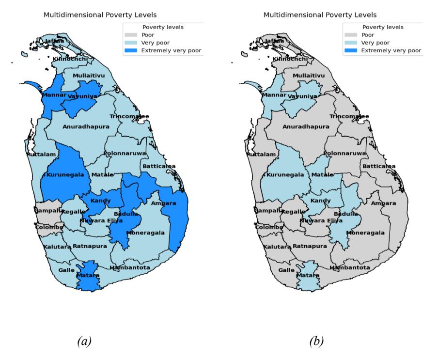
Figure 2 Spatial distribution of poverty level shifts (when N is low).
The results indicate that the Colombo and Gampaha districts show a 'poor' (P) level when compared to the other districts. Notably, there are seven instances classified as 'extremely very poor' (EVP) among households with low dependents, as illustrated in Figure 2(a). Colombo, Gampaha, Kalutara, Kandy, and Galle are recognized as the districts exhibiting the highest levels of urbanization in Sri Lanka [18].
The results illustrate that when the number of members of the household increases, Colombo and Gampaha's poverty levels shift to EVP and P levels, respectively (Figure 3(a)). The reason for this could be higher living standards, since those districts are urbanized and having more members in the households pushes them to more severe cases of poverty. Further, it can be observed that when the number of dependents increased, the EVP cases increased to 14 districts. When applying this scenario to districts with a high number of dependents, the analysis showed a worst-case outcome where all districts exhibited EVP cases.
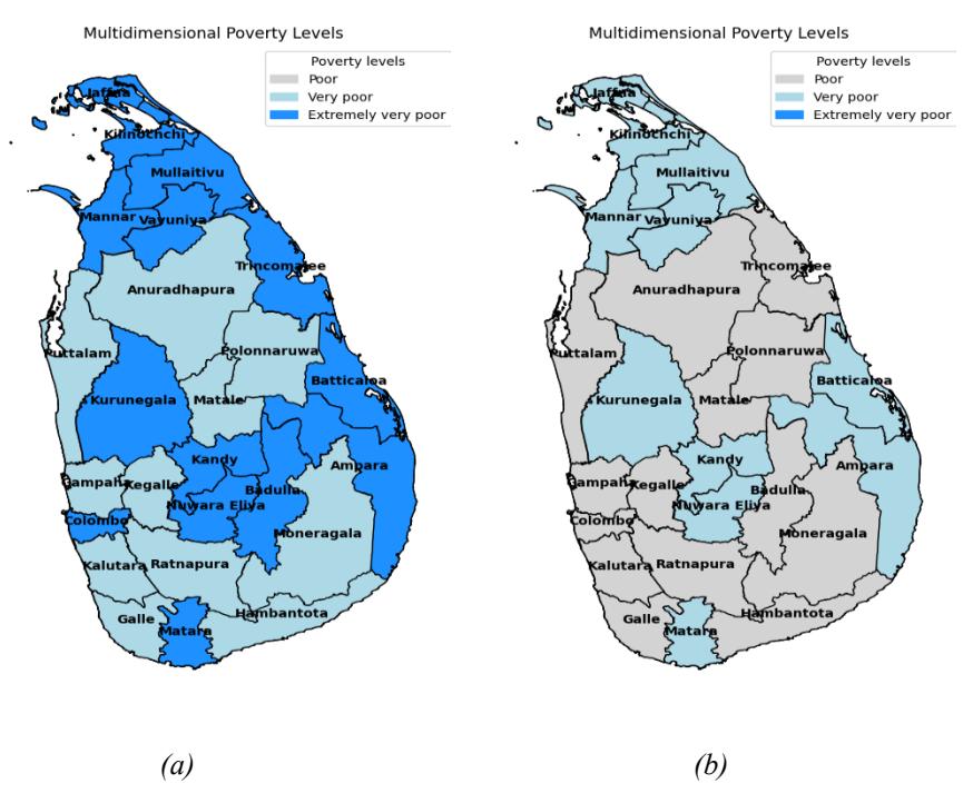
Figure 3 Spatial distribution of poverty level shifts (when N is medium).
Conversely, we observed that districts such as Monaragala, Rathnapura, Kegalle, Puttalam, Anuradhapura, Polonnaruwa, Hambantota, Galle, Matale, and Kaluthara did not exhibit significant shifts in poverty levels with increasing household size. This observation suggests that in these districts, increasing household members does not substantially impact poverty levels. One possible explanation is that households with a higher average number of children may have adapted better to larger household sizes compared to other districts [19].
We examined the impact of various factors on poverty reduction by individually altering each factor, Hs, I, and E, while allowing N and Ev to adjust accordingly. We did not apply the same increment or decrement of factors for all districts; instead, we did the analysis based on considering one district at a time. Therefore, Table 6 and Table 7 illustrate results generated from the model under scenarios where the number of dependents was varied to obtain corresponding poverty levels, while environmental vulnerability was maintained at a lower level for selected districts. For the remaining districts, environmental vulnerability was adjusted based on the available data, with emphasis on districts distributed across the Central, Western, Northern, Sabaragamuwa, and Southern provinces. These regions exhibit relatively higher environmental vulnerability and therefore we incorporated medium to high Ev inputs into our model.
Tabel 6 Poverty redemption levels for low N.
| Redemption levels | ||||
|---|---|---|---|---|
| District | Focused factor/s | level | ||
| Colombo | - | - | ||
| Gampaha | - | - | ||
| Kaluthara | Hs | Poor | ||
| Kandy | Hs | Very poor | ||
| Matale | Hs | Very poor | ||
| NuwaraEliya | E/Hs | Poor | ||
| Galle | Hs | Poor | ||
| Matara | Hs | Very poor | ||
| Hambanthota | Hs | Poor | ||
| Jaffna | E/Hs | Poor | ||
| Mannar | E/Hs | Very poor | ||
| Vavunia | E/Hs | Very poor | ||
| Mullative | E/Hs | Poor | ||
| Killinochchi | E/Hs | Poor | ||
| Batticaloa | Hs | Poor | ||
| Ampara | Hs | Poor | ||
| Trincomalee | E/Hs | Poor | ||
| Kurunegala | Hs | Very poor | ||
| Puttalam | Hs | Poor | ||
| Anuradhapura | Hs | Poor | ||
| Polonnaruwa | Hs | Poor | ||
| Badulla | E/Hs | Very poor | ||
| Monaragala | Hs | Poor | ||
| Rathnapura | E/Hs | Poor | ||
| Kegalle | Hs | Poor | ||
From the results in Table 6, it can be observed that poverty reduction is more significant in factors E and Hs. The EVP and VP cases shifted to VP and P levels compared to the previous results (Figure 2(b)). It can be observed that the most significant factor is Hs. Also, an increase in the educational attainment of the individuals has a positive impact on poverty reduction. When applying similar changes to the number of dependents, the results varied.
In districts such as Colombo, Badulla, and Trincomalee, poverty levels previously classified as EVP (Figure 3 (b)) were upgraded to the P level, with other districts also showing improvements to the P level. Again, Hs emerged as the most significant factor in these changes. According to the housing characteristics of the households, poverty reduction was more significant among almost all of the districts (Table 7).
Tabel 7 Poverty redemption levels for medium N.
| Redemption levels | |||||
|---|---|---|---|---|---|
| District | Focused factor/s | level | |||
| Colombo | - | - | |||
| Gampaha | I | Poor | |||
| Kaluthara | Hs | Poor | |||
| Kandy | Hs/I | Very poor/Poor | |||
| Matale | I | Poor | |||
| NuwaraEliya | Hs/I/E | Very poor/Very poor/Very poor | |||
| Galle | Hs | Poor | |||
| Matara | Hs/I | Very poor/Very poor | |||
| Hambanthota | Hs | Poor | |||
| Jaffna | Hs/I/E | Very poor/Poor/Very poor | |||
| Mannar | Hs/I/E | Very poor/Very poor/Very poor | |||
| Vavunia | Hs/I | Very poor/Very poor | |||
| Mullative | Hs/I/E | Very poor | |||
| Killinochchi | Hs | Very poor | |||
| Batticaloa | Hs/I | Very poor/Poor | |||
| Ampara | Hs/I | Very poor/Poor | |||
| Trincomalee | Hs/E | Poor | |||
| Kurunegala | Hs/I | Very poor/Poor | |||
| Puttalam | Hs | Poor | |||
| Anuradhapura | Hs | Poor | |||
| Polonnaruwa | I | Poor | |||
| Badulla | Hs/E | Poor | |||
| Monaragala | Hs/I | Poor | |||
| Rathnapura | Hs | Poor | |||
| Kegalle | Hs | Poor | |||
An increase in income only resulted in a decrease in poverty levels for Matale, Gampaha, and Polonnaruwa districts. In rural districts, our observations suggest that to effectively reduce poverty, at least the factors I, E, and Hs have to be more focused on. Table 7 contains the poverty level that each factor that could obtain. This provides a menu of focus factors to reduce poverty. Overall, the standard of living dimension has to be focused on for poverty reduction.
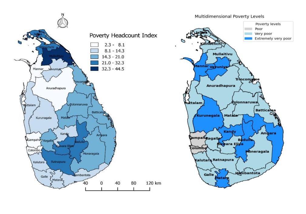
Source: HIES-2019 Department of Census and Statistics, Sri Lanka
From the model
Figure 4 Spatial distribution of poverty line vs MPI by district.
4 Validation results
Finally, the model was validated using the headcount ratio (HCR). This measure represents the proportion of individuals whose income lies below the defined poverty line. However, a key limitation of the HCR is its inability to capture poverty intensity; when the poor become poorer, the measure remains unchanged even as their conditions worsen [6]. Our model calculates the HCR by multiplying the HCR from the DCS by the sum of the degrees of each poverty level, as shown in Eq. (13). This approach enables us to identify poor households and determine which poverty level they belong to. The HCR for the model is calculated as follows:
Fuzzy headcount ration(FHCR) = \[HCR(P + VP + EVP)\]. (13)
Table 8 provides evidence that the proposed model performs effectively when income is considered and, at the same time, enables a multidimensional analysis of poverty. Figure 4 demonstrates that district-level poverty patterns differ substantially when comparing income-based poverty measures with multidimensional poverty indices, indicating that monetary indicators alone do not fully capture household deprivation.
Tabel 8 Validation results.
| District | Head count ratio (from | Headcount ratio (from the model) |
|---|---|---|
| DSC) | ||
| Colombo | 2.3 | 2.05 |
| Gampaha | 5.7 | 5.24 |
| Kaluthara | 12.2 | 11.35 |
| Kandy | 14.3 | 13.59 |
| Matale | 19.6 | 19.4 |
| NuwaraEliya | 26.3 | 24.2 |
| Galle | 13.2 | 12.01 |
| Matara | 11.1 | 10.43 |
| Hambanthota | 13.6 | 12.38 |
| Jaffna | 25.8 | 22.96 |
| Mannar | 8 | 7.6 |
| Vavunia | 13.9 | 13.07 |
| Mullative | 44.5 | 40.5 |
| Killinochchi | 26.4 | 23.5 |
| Batticaloa | 20.8 | 18.51 |
| Ampara | 17.2 | 17.2 |
| Trincomalee | 18.3 | 16.29 |
| Kurunegala | 12.5 | 11.88 |
| Puttalam | 10.5 | 9.45 |
| Anuradhapura | 8.1 | 7.29 |
| Polonnaruwa | 17 | 15.64 |
| Badulla | 32.3 | 31.33 |
| Monaragala | 21 | 19.11 |
| Rathnapura | 24.9 | 22.66 |
| Kegalle | 20.8 | 18.72 |
Based on the results, instead of treating all the districts equally, the government can make decisions or create policies to strengthen the districts that should prioritize reducing poverty. Mainly fiscal forms must be strengthened to reduce poverty and reinforce a household's educational attainment, such as investing in people and building human resources in society. Therefore, to minimize poverty education levels have to be focused on. It was observed that even urbanized and rural districts can fall to the worst poverty cases if the number of members in the households is high. Therefore, to empower the poor, policymakers can create subsidy distribution plans and resource allocation for the needy districts to improve the living standards of households in Sri Lanka.
5 Conclusion
This study presents a multidimensional approach to poverty classification. The results showed that the fuzzy approach enables the decomposition of the poverty levels of households, where the decomposition is based on the geographical characteristics of the country. This could be helpful when developing a poverty map of countries. In future work, we would like to apply this method to other developing countries and carry out further poverty classification.
6 References
- [1] Belhadj, B. & Bouanani, M., Attributes Inequality in Multidimensional Poverty Measures Fuzzy Modeling, Soft Computing, 27(4), pp. 1997-2008, 2023.
- [2] Asian Development Bank and World Bank, Climate Risk Country Profile: Sri Lanka, Available at: https://reliefweb.int/report/srilanka/climate-risk-country-profile-sri-lanka, 2020. [Accessed: July 13, 2023].
- [3] Department of Census and Statistics, Sri Lanka, Multidimensional Poverty Index: Brief, 2022. [Accessed June 18, 2023].
- [4] NASA, Extreme Weather, https://science.nasa.gov/climate-change/ extreme-weather/, 2024. [Accessed: May 15, 2024].
- [5] Marin, S.R., Glasenapp, S., de Almeida Vieira, C., Diniz, G.M., Porsse, M.D.C.S. & Ottoneli, J., Multidimensional Poverty in Silveira Martins/rs: An Application of Alkire-foster Method (af), Revista de Administração da UFSM, 11(2), pp. 247-267, 09 2018.
- [6] Ravallion, M., Issues in Measuring and Modelling Poverty, The Economic Journal, 106(438), pp. 1328-1343, 1996.
- [7] Peiris, H.O.W., Chakraverty, S., Perera, S.S.N. & Ranwala, S.M. W., Novel Fuzzy Linguistic Based Mathematical Model to Assess Risk of Invasive Alien Plant Species, Applied Soft Computing, 59, pp. 326- 339, 2017.
- [8] Klir, G. & Yuan, B., Fuzzy Sets and Fuzzy Logic, Prentice Hall, 1- 12, 1995.
- [9] Hasan, M.F. & Sobhan, M.A., Describing Fuzzy Membership Function and Detecting the Outlier by Using Five Number Summary of Data, American Journal of Computational Mathematics, 10(3), pp. 410-424, 2020.
- [10] Zimmermann, H.J., Fuzzy Set Theory and Its Applications, Springer Science & Business Media, 2011.
- [11] Belhadj, B., New Fuzzy Indices of Poverty by Distinguishing Three Levels of Poverty, Research in Economics, 65(3), pp. 221-231, 2011.
- [12] Karasan, A. & Erdogan, M., Creating Proactive Behavior for the Risk Assessment by Considering Expert Evaluation: A Case of Textile Manufacturing Plant, Complex & Intelligent Systems, 7(2), pp. 941-959, 2021.
- [13] Murty, R.L.N., Kondamudi, S.G., Suryanarayana, M.V. & Giribabu, P., Application of Buckley's Fuzzy AHP to Identify the Most Important Factor Affecting the Unorganized Micro-Entrepreneurs' Borrowing Decision, International Journal of Management (IJM), 11(6), pp. 665-674, 2020.
- [14] Jayathilaka, R., Joachim, S., Mallikarachchi, V., Perera, N. & Ranawaka, D., Do Chronic Illnesses and Poverty Go Hand in Hand?, PloS one, 15(10), e0241232, 2020.
- [15] Deyshappriya, N.R. & Feeny, S., Weighting the Dimensions of the Multidimensional Poverty Index: Findings from Sri Lanka, Social Indicators Research, 156(1), pp. 1-19, 2021.
- [16] Griliches, Z. & Mason, W.M., Education, Income, and Ability, Journal of Political Economy, 80(3), Part 2, pp. S74-S103, 1972.
- [17] ReliefWeb, Sri Lanka: Extreme Weather – Operation Update No. 1, DREF No. MDRLK015 – Sri Lanka, Available at: https://reliefweb.int/report/sri-lanka/sri-lanka-extreme-weatheroperation-update-ndeg-1-dref-ndeg-mdrlk015, 2022. [Accessed: July 13, 2023].
- [18] Weeraratne, B., Re-Defining Urban Areas in Sri Lanka, Institute of Policy Studies of Sri Lanka, 2016.
- [19] Department of Census and Statistics, Sri Lanka, Demographic and Health Survey 2016: Full Report, Available at: http://www.statistics.gov.lk/Health/StaticalInformation, 2016. [Accessed July 15, 2023].