
1 Introduction
Quantum computing is a recent advancement in the field of computing that helps to solve certain classes of complex problems faster than classical computers [1]. A landmark example is Shor's algorithm [14], proposed by Peter Shor in 1994, which provides exponential speedup over classical methods by solving the integer factorization problem. In 1996, Lov Grover introduced his well-known quantum search algorithm, designed to search for a marked element within an
Received January 30th, 2026, Revised February 9 th, 2026, Accepted for publication February 9 th, 2026 Copyright © 2026 Published by ITB Institut for Research and Community Service, ISSN: 2337-5760, DOI: 10.5614/j.math.fund.sci.2026.57.3.2
1 Selected paper from International Conference on Computational and Mathematical Modelling (ICCMM) 2025 in Sri Lanka
unsorted database. In particular, this offers a quadratic speedup, achieving a time complexity of (√) compared to the classical search time complexity of ().
Quantum walks are a key concept in quantum computing that provides a platform for devising quantum algorithms, particularly for graph-related problems. It is the quantum-mechanical counterpart of the classical random walk, which is described through the evolution of a quantum particle (walker) [7]. A classical random walker starts from an initial vertex and its movement is governed by an unbiased coin [15]. If the outcome is head, the walker moves to the right-adjacent vertex; if it is tail, it moves to the left-adjacent vertex [1]. In contrast to this, the evolution of a quantum walker is governed by two operators: the coin operator () and the shift operator (). The combination of these two operators results in a unitary evolution operator = ⊗ . The walker is initially in the state |n⟩ and after the coin operator is applied, a portion of the walker is reserved for |n + 1⟩, and another portion is reserved for |n − 1⟩ [1], implying that the coin operator creates the superposition state. When S is applied, these portions are transmitted to the corresponding states. In other words, the shift operator updates the position of the walker. If the Grover operator () is used as the coin operator, it will describe the dynamics of the Grover walk.
The Grover walk is a discrete-time quantum walk (DTQW) model inspired by Grover's algorithm. Previous studies have explored the dynamics of the Grover walk in the context of Johnson graphs [5] and hypercubes [13]. In recent years, many other graph topologies have been considered [9]. Higuchi et al. [3] proposed a novel quantum walk model with in- and out-flows on complete graphs, addressing the 'soufflé problem' of oscillating probabilities. Their framework treats the complete graph () as an internal graph connected to semiinfinite tails, enabling convergence to a stationary state. It has been shown that the transition matrix (Eq. (7)) for any complete graph can be modeled by a 3 × 3 matrix. They used Kato's perturbation theory [11] to approximate the eigenvalues of . The study concluded that the quantum walk can find the marked vertex with a high probability (>1/2) in the stationary state.
The primary objective of our study is to investigate the behavior and performance of Grover's quantum walk on cyclic graphs. Initially, the probability of detecting the marked vertex is set to zero. Subsequently, using Eqs. (5) and (6), the probability is computed iteratively at each time step. It enables visualization of the probability distribution of the marked vertex over time. Finally, the stationary state is identified and the long-term probability of detecting the marked vertex is determined.
This paper is organized as follows: Section 2 presents the methodology and is divided into three subsections: the Grover walk on \(C_6\); the Grover walk on general odd cycle; and the Grover walk on a general even cycle. Section 3 discusses the results obtained from the study. Finally, Section 4 presents the conclusions and potential directions for future research.
2 Methodology
The study starts with the simplest case, the 3-cycle. It is already known that Grover's search performs well on complete graphs with connected tails [3]. Since \(C_3\) is a complete graph, the Grover search is effective on it. Also, Sabri and Sahabandu [4] showed that Grover search performs well on \(C_4\) and \(C_5\). Hence, we initiate our study with \(C_6\) and then this approach is generalized to \(C_N\).
2.1 Grover Walk on \(C_6\)
In this section, we fix the internal graph as a cyclic graph with six vertices. Let \(\{P_j: j=1,2,...,6\}\) be the set of tails whose end vertex is denoted by \(e(P_j)\) and the set of vertices of \(C_6\) be \(\{u_j: j=1,2,...,6\}\). Then we connect the tail \(P_j\) to the vertex \(u_j\) with \(e(P_j)\), as shown in Figure 1. The resulting graph is denoted by \(\tilde{C}_6\). Each edge is replaced with a pair of arcs that are symmetric and have opposite directions. Let A and \(\tilde{A}\) be the arc set induced by the set of edges \(E(C_6)\) and \(E(\tilde{C}_6)\), respectively. For each arc \(a \in \tilde{A}\) from the vertex u to vertex v, we denote u by the origin of a; u = o(a) and v by the terminal of a; v = t(a) [3]. Each arc \(a \in \tilde{A}\) represents a probability amplitude of the quantum state.
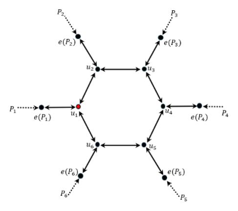
Figure 1 A semi-infinite tail (path) is attached to each vertex of \(C_6\). The labels \(u_1, u_2, ..., u_6\) denote cycle vertices.
2.1.1 Role of Tails
According to the model in [3], attaching semi-infinite tails to a finite graph prevents the probability from oscillating forever (the 'soufflé problem' in closed quantum walks). On a finite cycle without tails, the walk is closed. Consequently, the probability at any vertex does not settle to a fixed value. To obtain a stationary distribution, we attach a tail to every vertex of \(C_N\). This creates an open quantum system: at each step, a fixed unit of amplitude flows into the cycle from the tails (inflow). Any amplitude that enters a tail flows outward to infinity and never returns (outflow). The balance of inflow and outflow allows the system to converge to a stationary state.
In Grover's quantum walk, the coin operator is given by the Grover operator \(G(r) = (2/r)J_r - I_r\) [3], where r is the degree of the vertex on which the Grover operator is applied. The matrices \(J_r\) and \(I_r\) are the all-one matrix and the identity matrix, respectively. The Hilbert space \(H_{\tilde{A}}\) of the coined model associated with \(C_N\) is spanned by the set of arcs, that is, \(H_{\tilde{A}} = span\{|a\rangle: a \in \tilde{A}\}\) [5]. The dimension of \(H_{\tilde{A}}\) is \(|\tilde{A}| = 2|E(\tilde{C}_N)|\). The shift operator, denoted by S, acts as \(S|a\rangle = |\bar{a}\rangle\) [1], where \(\bar{a}\) is the inverse arc of a.
Let \(\{a_1, a_2, a_3, ..., a_r\}\) be the subset of \(\tilde{A}\) such that \(u = t(a_i)\): i = 1,2,3,...,r where \(u \in V(C_N)\) is an arbitrary vertex. As each vertex in the cycle with the tails has a degree of 3, we conclude that r remains constant at 3. Let \(a_{i,t}\) be the amplitude in arc \(a_i\) at time step t. In the Grover search, the oracle identifies the marked element by multiplying its state by -1. We use the same mechanism in the coined walk. According to Higuchi et al. [3], the recursion given in Eq. (1) holds.
\[\text{[rumus tidak dapat ditampilkan dengan baik — lihat PDF asli]}\]
2.1.2 Initial State
The first step is to label the arcs. As shown in Figure 2(a), \(C_6\) is symmetric over the dotted line. That enables the arcs to be labeled symmetrically. In this model, the initial amplitudes are placed only on the arcs coming from the attached tails into the cycle. Let \(u_1\) be the marked vertex. The initial state \(\psi_0\) is set according to [3] as follows:
\[\psi_0(a) = \begin{cases} 1, & \text{if } a \in (\tilde{A} \setminus A) \text{ and } \operatorname{dist}(\mathsf{t}(a), C_N) < \operatorname{dist}(\mathsf{o}(a), C_N) \\ 0, & \text{otherwise} \end{cases}\] (2)
Since the vertices of \(C_N\) have a distance 0 to the cycle and the tail vertices have a positive distance, the above condition initializes the walk with a unit inflow into each vertex of \(C_N\).
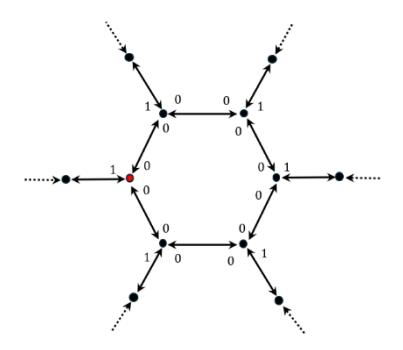
(a) Symmetric labeling of arcs on C<sub>6</sub> with the marked vertex \(u_1\). The dashed lines indicate the symmetry axis used for labeling.
(b) Initial state—unit amplitude (inflow) is placed on each tail arc pointing into the cycle, while all other arcs have zero amplitude.
Figure 2 Setting up the system.
System of Recursions for Grover Dynamics
The Grover walk can be modeled using the transition rate and the reflection rate [1]. The transition rate is defined as \(\frac{2}{\deg(u)}\), where \(\deg(u) = \deg(u)\) degree of vertex u. The reflection rate is defined as \(\frac{2}{\deg(u)} - 1\).
Let a be the probability amplitude in arc \((v_1, u)\) at time t. Figure 3(a) shows the case where \(u \neq u^*\). In the next iteration, the amplitudes split as follows:
- Transmitted portions <sup>2</sup>/<sub>3</sub> a moving to vertices v<sub>2</sub> and v<sub>3</sub> Reflected portion <sup>1</sup>/<sub>3</sub> a returning to vertex v<sub>1</sub>
Figure 3(b) illustrates the marked vertex scenario, where the signs of the rates are inverted according to Eq. (1). Hence, the transmitted portion becomes \(-\frac{2}{3}a\) and the reflected portion becomes \(\frac{1}{3}a\).
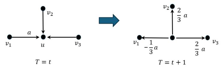
(a) ≠ ∗ : For an unmarked vertex, an incoming amplitude splits into a reflected portion − 1 3 and transmitted portions 2 3 .
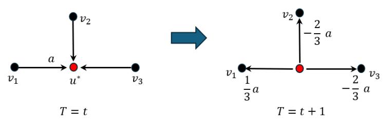
(b) = ∗ : For the marked vertex, the signs are inverted; reflected portion 1 3 and transmitted portions − 2 3 .
Figure 3 Transition and reflection of a probability amplitude on a vertex .
Based on Figure 4, the recursive system is derived with the initial conditions specified in Eq. (2). Let , , where ∈ {1,2, … ,6} denotes the amplitude in arc at time step . We derive recursive relations for each , based on the amplitudes from the previous iterations.
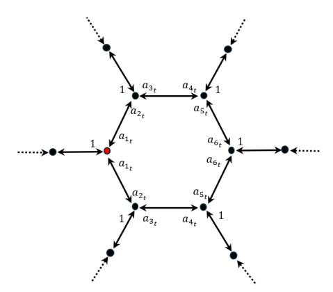
Figure 4 Labeling of the arcs around 6 used to derive recursive amplitude relations.
The Grover coin for degree 3 yields a reflection rate of -1/3 and a transition rate of +2/3 for unmarked vertices, with signs inverted for the marked vertex.
Consider the arc \(a_{1_t}\), which points from \(u_2\) to \(u_1\). Its amplitude at time t receives three contributions from time t-1 as follows:
- 1. Tail inflow From the tail attached to \(u_2\), contributing a constant amplitude 2/3
- 2. Reflection from \(a_{2_t}\) Arc \(a_{2_t}\) pointing to \(u_2\) reflects with rate -1/3
- 3. Transmission from \(a_{3_t}\) Arc \(a_{3_t}\) pointing to \(u_2\) transmits to \(u_1\) with rate 2/3
Thus, the following recurrence holds:
\[a_{1,t} = \frac{2}{3} - \frac{1}{3}a_{2,t-1} + \frac{2}{3}a_{3,t-1}\]
\((a_{1,t} = \text{transition of } \psi_{t-1}(l) + reflection of \; \psi_{t-1}(b) + transition of \; \psi_{t-1}(c))\) [see Figure 2(a)].
Similarly, we derive recursion formulas for each \(a_{i,t}\) as follows:
\[a_{2,t} = -\frac{2}{3} + \frac{1}{3}a_{1,t-1} - \frac{2}{3}a_{1,t-1}\]: constant term \(-2/3\) is the contribution of arc \(g = -\frac{2}{3} + \frac{1}{3}a_{1,t-1}\)
\((a_{2,t} = \text{transition of } \psi_{t-1}(g) + reflection of \psi_{t-1}(a) + transition of \psi_{t-1}(a))\)
\[a_{3,t} = \frac{2}{3} - \frac{1}{3} a_{4,t-1} + \frac{2}{3} a_{5,t-1}: \text{ constant term 2/3 is the contribution of arc } i\] \[a_{4,t} = \frac{2}{3} + \frac{2}{3} a_{2,t-1} - \frac{1}{3} a_{3,t-1}: \text{ constant term 2/3 is the contribution of arc } h\] \[a_{5,t} = \frac{2}{3} + \frac{1}{3} a_{6,t-1}: \text{ constant term 2/3 is the contribution of arc } j\] \[a_{6,t} = \frac{2}{3} + \frac{2}{3} a_{4,t-1} - \frac{1}{3} a_{5,t-1}: \text{ constant term 2/3 is the contribution of arc } k\] (3)
The constant terms in the recursion formulas arise from the inflow of amplitude from the attached tails. The system of equations is expressed in matrix form as:
\[\psi_t = A\psi_{t-1} + B, \quad \psi_0 = 0 \tag{4}\]
Where \[\psi_t = \begin{pmatrix} a_{1t} \\ a_{2t} \\ a_{3t} \\ a_{4t} \\ a_{5t} \\ a_{6t} \end{pmatrix}\], coefficient matrix \(A = \begin{bmatrix} 0 & -\frac{1}{3} & \frac{2}{3} & 0 & 0 & 0 \\ -\frac{1}{3} & 0 & 0 & 0 & 0 \\ 0 & 0 & 0 & -\frac{1}{3} & \frac{2}{3} & 0 \\ 0 & 0 & 0 & 0 & \frac{1}{3} & \frac{2}{3} & 0 \\ 0 & 0 & 0 & 0 & \frac{2}{3} & -\frac{1}{3} & 0 & 0 \\ 0 & 0 & 0 & 0 & \frac{2}{3} & -\frac{1}{3} & 0 \end{bmatrix}\)
and constant vector \[B = \begin{pmatrix} 2/3 \\ -2/3 \\ 2/3 \\ 2/3 \\ 2/3 \end{pmatrix}\].
2.1.4 Computation of the Probability of Locating the Marked Vertex
First, we determine the relative probability of each vertex, as described by the formula in [3]. The relative probability of finding a vertex \(u \in V(C_N)\) in the \(t^{th}\) iteration is given by the following equation:
\[\tilde{p}_t(u) = \sum_{t(a)=u} |\psi_t(a)|^2 \tag{5}\]
The probability of finding the marked vertex \(u^*\) is obtained by normalizing the relative probability, as follows:
\[p_t(u^*) = \frac{\tilde{p}_t(u^*)}{\sum_{u \in V(C_N)} \tilde{p}_t(u)}\] (6)
From Eq. (5), the relative probability of finding the marked vertex \(u_1\) at the first iteration is calculated as \(\tilde{p}_1(u_1) = |\psi_1(a)|^2 + |\psi_1(a)|^2 = 2|\frac{2}{3}|^2 = \frac{8}{9}\). Note that the relative probabilities of all vertices are the same after the first iteration. Thus, by Eq. (6), the probability of finding the marked vertex after the first iteration is computed as \(p_1(u_1) = \frac{8/9}{6(8/9)} = \frac{1}{6} = 0.1666\). Since the relative probabilities are identical for all vertices, the probability of locating any specific vertex becomes uniform. Consequently, after the first iteration, the system evolves into a state of equal superposition. This behavior is not exclusive to the \(C_6\), but generally holds for any cyclic graph.
It is observed that the system of equations (4) allows the computation of amplitude values for each iteration. Figure 5 illustrates how the probability of the marked vertex varies with the number of iterations.
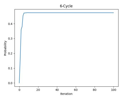
Figure 5 Probability distribution of the marked vertex over the successive iterations for \(C_6\).
2.1.5 Stationary State
According to Higuchi and Segawa [6], \(\lim_{t\to\infty} \psi_t\) exists; we denote it by \(\psi_{\infty}\). We call \(\psi_{\infty}\) the stationary state. Taking the limit of Eq. (4), we obtain the following:
\[\lim_{t \to \infty} \psi_t = \lim_{t \to \infty} A \psi_{t-1} + B\] \[\psi_{\infty} = A \psi_{\infty} + B\] \[(I - A) \psi_{\infty} = B\] \[\psi_{\infty} = (I - A)^{-1} B\]
Solving this system for \(\psi_{\infty},\) we get the normalized stationary state for \(\mathcal{C}_{6}\) as
\[\psi_{\infty} = \frac{3}{\sqrt{76}} \begin{bmatrix} 2\\ -4/3\\ 4/3\\ -2/3\\ 2/3\\ 0 \end{bmatrix}.\]
Applying Eq. (5), the relative probability of finding \(u^*\) in the long run is given by \(2|\psi_\infty(1)|^2=2|\frac{3}{\sqrt{76}}\times 2|^2=2\times\frac{9}{19}=\frac{18}{19}\). The total relative probability over all six vertices is \(\sum_u \tilde{p}_\infty(u^*)=2\sum_{i=1}^6 |\psi_\infty(i)|^2=2\|\psi_\infty\|=2\times 1=2\). Applying the formula in Eq. (6) to the stationary relative probabilities, we obtain the long-run probability \(P(u^*)=\frac{18}{38}=0.47368\).
2.2 Grover Walk on General Odd Cycle
In this section, we fix the internal graph as a cyclic graph with an odd number of vertices, denoted by \(C_{N_{odd}}\). As described in Section 2.1, tails are attached to each of the vertices in \(C_{N_{odd}}\); the resulting graph is shown in Figure 6.
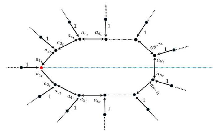
Figure 6 Tail attachment and amplitude labeling for a general odd cycle \(C_{N_{odd}}\), showing the probability amplitudes at time step t.
Following the methodology outlined in Section 2.1.3, we derive the recursion systems for \(C_3\), \(C_5\), \(C_7\), and \(C_9\) separately and obtain the corresponding coefficient matrix \(A_i\) for each of these cycles. By analyzing these matrices, we observed a recurring pattern and construct an algorithm to determine the coefficient matrix \(A_{N \times N}\) for any general odd cycle. The algorithm is presented below:
Let N be the number of vertices in \(C_{N_{odd}}\), and \(n \in \{1,2,3,...,N\}\).
\[a_{2,t} = -\frac{2}{3} - \frac{1}{3}a_{1,t-1}\] \[a_{N,t} = \frac{2}{3} + \frac{2}{3}a_{N-1,t-1} - \frac{1}{3}a_{N,t-1}\] if n is even and n > 2,
\[a_{n,t} = \frac{2}{3} + \frac{2}{3}a_{n-2,t-1} - \frac{1}{3}a_{n-1,t-1}\] if n is odd and n < N,
\[a_{n,t} = \frac{2}{3} - \frac{1}{3}a_{n+1,t-1} + \frac{2}{3}a_{n+2,t-1}\]
The pseudocode below summarizes the construction procedure.
Input: N (Odd integer, N > 2) Output:
×
BEGIN
  A ← zero matrix of size N ×N
  FOR  = 1 TO  DO
    IF (n is even) AND ( > 2) THEN
        A[n][n−2] ← 2/3
        A[n][n−1] ← −1/3
    ELSE IF (n is odd) AND (n < N) THEN
        A[n][n+1] ← −1/3
        A[n][n+2] ← 2/3
    END IF
  END FOR
  // Special fixed entries
        A[2][1] ← −1/3 // Row 2, Column 1
        A[N][N −1] ← 2/3 // Row N, Column N-1
        A[N][N] ← −1/3 // Row N, Column N
  RETURN A
END
Following a similar methodology for the complete graph [3], we set = , where the matrix = [ √2 0 0 0 √2 0 0 0 √2 … 0 … 0 … 0 0 0 0 0 0 0 … 0 … √2] = √2 and
= [1 , 2 , … . , ] . From Eq. (4), we derive+1 as follows:
\[\alpha_{t+1} = Z\psi_{t+1}\] \[= Z(A\psi_t + B)\] \[= ZA\psi_t + ZB\] \[= (ZAZ^{-1})(Z\psi_t) + (ZB)\] \[\alpha_{t+1} = T\alpha_t + b, \alpha_0 = 0\] (7)
By computing the matrix , we obtain = −1 = √2 1 √2 = . For the complete graph, the elements of the matrix depend on the number of vertices [3].
According to [3], the eigenvalues T were approximated using the perturbation theorem. Nevertheless, for cyclic graphs, the elements of T do not depend on N, since each vertex in the cyclic graph with attached tails has a degree of 3, which is independent of N. Therefore, the perturbation theorem is not applicable in this case.
Note that from Eq. (7), we obtain \(\alpha_0 = 0\), \(\alpha_1 = b\), \(\alpha_2 = Tb + b\), \(\alpha_3 = T(Tb + b) + b = (T^2 + T + I)b\), and in general, \(\alpha_t = (T^{t-1} + T^{t-2} + \dots + T + I)b\). Diagonalizing the matrix T, such that \(T = PDP^{-1}\), where D is the diagonal matrix whose diagonal elements are eigenvalues of T and P, is the matrix whose columns consist of the eigenvectors corresponding to those eigenvalues. Consequently, we have
\[\alpha_t = P(D^{t-1} + D^{t-2} + \dots + D + I)P^{-1}b\] (8)
Let \(\lambda_1, \lambda_2, \lambda_3, ..., \lambda_N\) be the eigenvalues of T. Then the matrix \(D^{t-1} + D^{t-2} + ... + D + I\) can be written as:
\[\begin{bmatrix} \lambda_1^{\,t-1} + \cdots + \lambda_1 + 1 & 0 & 0 & 0 & 0 \\ 0 & \lambda_2^{\,t-1} + \cdots + \lambda_2 + 1 & 0 & \dots & 0 \\ 0 & 0 & \lambda_3^{\,t-1} + \cdots + \lambda_3 + 1 & 0 & 0 \\ 0 & 0 & 0 & \dots & 0 \\ 0 & 0 & 0 & 0 & \lambda_N^{\,t-1} + \cdots + \lambda_N + 1 \end{bmatrix}\]
By taking the summation of the geometric series and substituting the result into Eq. (8), we derive the following system:
\[\alpha_t = P \begin{bmatrix} \frac{1-\lambda_1^{\ t}}{1-\lambda_1} & 0 & 0 & \dots & 0 \\ \frac{1-\lambda_1^{\ t}}{1-\lambda_2} & \frac{1-\lambda_2^{\ t}}{1-\lambda_2} & 0 & \dots & 0 \\ 0 & 0 & \frac{1-\lambda_3^{\ t}}{1-\lambda_3} & 0 & 0 \\ 0 & 0 & 0 & \dots & \frac{1-\lambda_N^{\ t}}{1-\lambda_N} \end{bmatrix} P^{-1}b\]
The existence of the limit \(\alpha_{\infty}\) in Eq. (9) is guaranteed by the general theory of quantum walks with tail inflows [6], where T corresponds to the operator \(E_{PON}\). In the notation of [6], the subspace \(H_u\) (eigenvalues with \(|\lambda| > 1\)) is always empty. Nevertheless, the subspace \(H_c\) (eigenvalues with \(|\lambda| = 1\)) may be nonempty, and eigenvalues with \(|\lambda| < 1\) are also present. Their proof shows that \(H_c\) being non-empty does not affect the convergence for the following reasons:
• The initial state lies in \(H_s\), the subspace spanned by eigenvectors whose eigenvalues satisfy \(|\lambda| < 1\) (Lemma 3.5).
• The subspaces \(H_c\) and \(H_s\) are orthogonal (Lemma 3.4).
Consequently, the repeated action of \(E_{PON}\) on the initial state remains entirely within \(H_s\), where all eigenvalues satisfy \(|\lambda| < 1\), and this guarantees the convergence. In our specific setting, we observe that numerically all eigenvalues indeed satisfy \(|\lambda| < 1\). We computed the spectrum of \(T_N\) for various cycles. Table 1 summarizes the results as follows:
Table 1 Spectral radius \(\rho(T_N)\) of the transition matrix \(T_N\) for various cycles. All values satisfy \(\rho(T_N) < 1\), ensuring convergence to a stationary state. The spectral radius increases with N and approaching 1 as \(N \to \infty\).
| \(C_N\) | \(\rho(T_N)\) |
|---|---|
| \(C_3\) | 0.7101 |
| \(C_4\) | 0.4387 |
| \(C_5\) | 0.8398 |
| \(C_6\) | 0.4898 |
| \(C_7\) | 0.8986 |
| : | : |
| \(C_{1000}\) | 0.99996 |
Since \(|\lambda_i| < 1\) for all eigenvalues of T, it follows that \(\lim_{t \to \infty} \lambda_i^t = 0\). Taking the limit \(t \to \infty\) on both sides, we obtain the following:
\[\lim_{t \to \infty} \alpha_t = \lim_{t \to \infty} P \begin{bmatrix} \frac{1 - \lambda_1^t}{1 - \lambda_1} & 0 & 0 & \dots & 0 \\ \frac{1 - \lambda_1}{1 - \lambda_2} & \frac{1 - \lambda_2^t}{1 - \lambda_3} & 0 & 0 & 0 \\ 0 & 0 & \frac{1 - \lambda_3^t}{1 - \lambda_3} & \dots & 0 \\ 0 & 0 & 0 & 0 & \frac{1 - \lambda_N^t}{1 - \lambda_N} \end{bmatrix} P^{-1} b\]
\[\alpha_{\infty} = P \begin{bmatrix} \frac{1}{1-\lambda_{1}} & 0 & 0 & \dots & 0\\ \frac{1}{1-\lambda_{1}} & \frac{1}{1} & 0 & 0 & 0\\ 0 & \frac{1}{1-\lambda_{2}} & \frac{1}{1} & 0 & 0\\ 0 & 0 & \frac{1}{1-\lambda_{3}} & \dots & 0\\ 0 & 0 & 0 & 0 & \frac{1}{1-\lambda_{N}} \end{bmatrix} P^{-1}b\]
From Eq. (9), we can compute the stationary state \(\alpha_{\infty}\). The relative probability of finding \(u^*\) in the long run is given by \(|\alpha_{\infty}(1)|^2\).
2.3 Grover Walk on General Even Cycle
We now fix the internal graph as a cyclic graph with an even number of vertices, denoted by . As described in Section 2.2, we attach the tails to each of ∈ ( ). Figure 7 shows the probability amplitude at the time step .
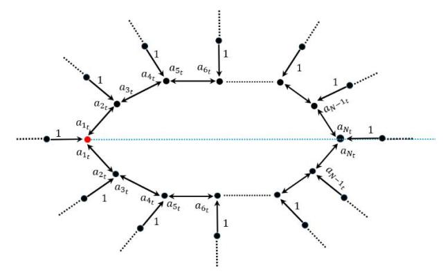
Figure 7 Tail attachment and amplitude labeling for a general even cycle .
Similar to the case of odd cycles, we observed a recurrent pattern in the elements of the coefficient matrices and derived an algorithm to determine the coefficient matrix × for any even cycle.
Let be the number of vertices in and ∈ {1,2,3, … , }.
\[a_{2,t} = -\frac{2}{3} - \frac{1}{3} a_{1,t-1}\]
\[a_{N-1,t} = \frac{2}{3} + \frac{1}{3} a_{N,t-1}\] if n is even and > 2,
\[a_{n,t} = \frac{2}{3} + \frac{2}{3}a_{n-2,t-1} - \frac{1}{3}a_{n-1,t-1}\] if n is odd and < − 1,
\[a_{n,t} = \frac{2}{3} - \frac{1}{3}a_{n+1,t-1} + \frac{2}{3}a_{n+2,t-1}\]
The pseudocode below summarizes the construction procedure.
Input:  (Even integer,  > 2)
Output: ×
BEGIN
  A ← zero matrix of size  ×
  FOR  = 1 TO N DO
    IF (n is even) AND (n > 2) THEN
        A[n][n−2] ← 2/3
        A[n][n−1] ← −1/3
    ELSE IF (n is odd) AND (n < N-1) THEN
        A[n][n+1] ← −1/3
        A[n][n+2] ← 2/3
    END IF
  END FOR
  // Special fixed entries
        A[2][1] ← −1/3 // Row 2, Column 1
   A[N-1][N] ← 1/3 // Row N-1, Column N
  RETURN A
END
As detailed in Section 2.2, we arrive at the same system as represented in Eqs. (7), (8), and (9).
3 Results and Discussion
This section presents the probability distribution for finding the marked vertex across cycles of varying sizes. We analyze how the probability evolves over successive iterations and compare its behavior across different cycles. Furthermore, we examine the effect of varying the number of iterations to understand the long-term behavior of the distribution.
Figure 8(a) shows a peak at a time step of 2, where the probability value is 0.6923. In Figure 8(b), a peak occurs at time step 3, with a probability value of 0.5833. Similarly, Figure 8(c) shows a peak with probability 0.5588. In each of these cases, the probability value remains greater than 0.5. Nevertheless, after 5, the probability value falls below 0.5.
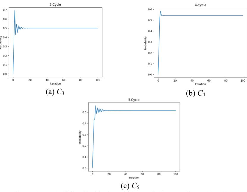
Figure 8 Probability distribution of the marked vertex in small cycles 3 − 5 .
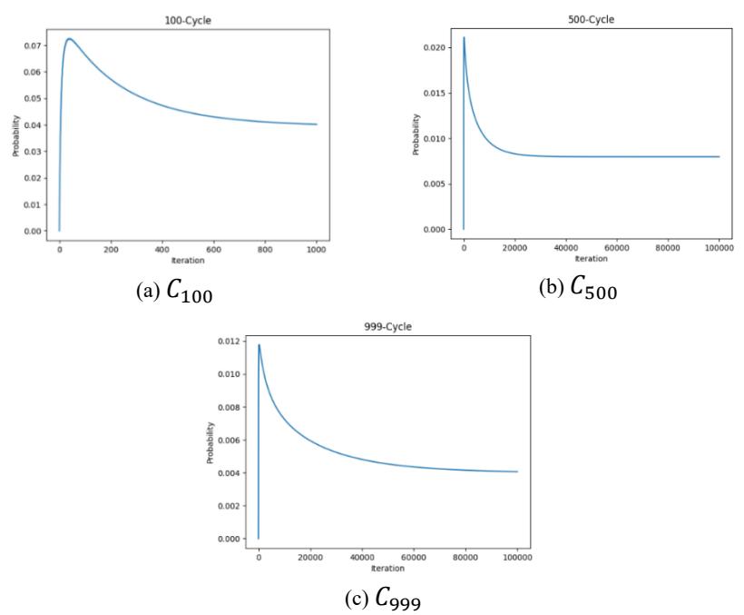
Figure 9 Probability distribution of the marked vertex in large cycles 100, 500, and 999.
Figures 8 and 9 illustrate that the probability distribution converges to a specific value. We now determine the stationary state using Eq. (9) and examine the probability of finding the marked vertex in this state. Consider the cycle \(C_3\). As described in Section 2.2, we obtain the eigenvalues of \(A_3\) as \(\lambda_1 = 0.1884 + 0.3478i\), \(\lambda_2 = 0.1884 - 0.3478i\), and \(\lambda_3 = -0.7101\). According to Eq. (9), we write the stationary state as follows:
\[\alpha_{\infty} = P \begin{bmatrix} \frac{1}{1-\lambda_1} & 0 & 0\\ 0 & \frac{1}{1-\lambda_2} & 0\\ 0 & 0 & \frac{1}{1-\lambda_3} \end{bmatrix} P^{-1}\,,\] where \[P = \begin{bmatrix} -0.6308 & -0.6308 & -0.7235\\ 0.2532 - 0.4674i & 0.2532 + 0.4674i & -0.3396\\ -0.0517 - 0.5628i & -0.0517 + 0.5628i & -0.6009 \end{bmatrix}.\]
Finally, we obtain normalized stationary state \(\alpha_{\infty} \approx \frac{1}{\sqrt{2}} \begin{bmatrix} 1 \\ -1 \\ 0 \end{bmatrix}\). According to Eq. (6), we get the probability of finding \(u^*\) in the long run as \(P_{\infty}(u^*) = \frac{|\alpha_{\infty}(1)|^2}{\sum_{i \in \{1,2,3\}} |\alpha_{\infty}(i)|^2} = \frac{1/2}{1} = \frac{1}{2}\). Similarly, the probability of \(u^*\) in the long run can be determined for any cycle. Table 2 illustrates the corresponding long-run probability values for various cycles.
Table 2 Long-run probability \(p_{\infty}(u^*)\) of finding the marked vertex for cycles \(C_3\) to \(C_7\) and for large cycles \(C_{1000}\). The probability exceeds 0.5 only for very small cycles \((C_4, C_5)\) and decays toward zero as N increases.
| Type of the cycle | \(p_{\infty}(u^*)\) |
| \(C_3\) | 0.5 |
| \(C_4\) | 0.5435 |
| \(C_5\) | 0.5158 |
| \(C_6\) | 0.4737 |
| C7 | 0.4321 |
| : | : |
| \(C_{1000}\) | 0.0039 |
Figure 10 shows the probability of finding the marked vertex in the long run with respect to the number of vertices (N) in the cycle. The graph illustrates how this probability changes as the size of the cyclic graph increases. We observe that the probability of finding the marked vertex decreases as the number of vertices in the cycle increases, and ( ∗ ) → 0 as → ∞. The cyclic structure degrades the search probability because the walker's amplitude spreads symmetrically in both directions along the cycle. This contrasts with the complete graph, where high connectivity enables efficient amplitude reflection and a high success probability.
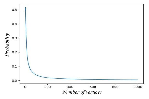
Figure 10 Probability of finding ∗ in the long-run over the number of vertices (). The probability decays asymptotically to zero as → ∞, illustrating the fundamental limitation of Grover-search-based quantum walks on cyclic graphs.
4 Conclusion
Grover's search algorithm has proven to be effective for various types of graphs, including complete graphs and Johnson graphs. The main objective of this study was to investigate the behavior and performance of Grover's quantum walk on cyclic graphs, with a focus on understanding how the probability of finding the marked vertex varies with the size of the cycle. In previous studies, perturbation theory was used to approximate the eigenvalues of the transition matrix (Eq. (7)) when the elements of the matrix are dependent on the number of vertices . In contrast, perturbation theory could not be applied in this study, since the elements of transition matrix T are independent of N. Therefore, in this case, we obtained eigenvalues directly.
Figure 8 shows that the search algorithm performs more effectively on smaller cyclic graphs such as 3, 4, and 5. In these cases, the probability of finding the marked vertex exceeds 0.5. Nevertheless, as the size of the cyclic graph increases, the effectiveness of the search algorithm decreases. For larger cycles, such as 500 and 999, the probability of finding the marked vertex decreases
significantly. This observation aligns with theoretical expectations, as the complexity of the search problem grows with the size of the graph.
This study had certain limitations. One significant limitation is the inability to define the coefficient matrix mathematically for a general cyclic graph. We developed an algorithm to construct for specific cases, yet a general mathematical expression for could not be derived. As a result, we were unable to derive the time complexity of the algorithm for general cyclic graphs. Given that the success probability tends to zero as the number of vertices increases, an interesting direction for future research is to explore Tulsi's modification method (Chapter 9 in [1]). Tulsi's approach aims to define a new unitary operator that maintains the same running time as the original Grover's algorithm while achieving a constant success probability, even as the size of the graph grows.