
1 Introduction
Saguling GBU operates only when demand for electricity occurs. Fast response time (2 minute) from non operating state to connected state has become an advantage for Saguling plant compare to similar plant with different generating source. The plant also contribute in maintaining transmission system frequency stability, besides its main role to produce electricity [1].
Generally, in order to transmit voltage and at the same time maintain frequency stability, hydro powerplant must be connected to the transmission system. For that purpose, the plant frequency must be made equal to the transmission system frequency. This sequence is done manually. Once it is connected, the whole process, including electricity producing, is done automatically.
Controller is modeled and designed with hope that it would increase plant's performance rather than controlled manually. The criterion chosen to evaluate plant's performance are settling time and the existence of maximum overshoot. The basic consideration for choosing these criterions is because system response is clearly seen based on these criterions. In addition, at present time, system response still has overshoot and long duration of settling time. System is modeled using neural network with backpropagation algorithm while Model Predictive Control is used to designed the controller.
2 Hydro Powerplant Fundamentals
2.1 Basic Principle
Frequency is a significant aspect in hydro powerplant. Initially, frequency has to be made synchronized with the transmission system frequency, which is 50 Hz. Once it is connected, plant's frequency will be influenced by transmission system frequency due to small capacity in power production that the plant's generate, relative to overall power consumption [2]. If there is an increasing in demand for electrical power, there will be an increasing in amount of power transferred from the powerplant as well. Plant's frequency will gradually decreased in result. This frequency fluctuation will affect the turbine angular speed.
2.2 Control Principle
Hydro powerplant has two sequence of control, there are control in start up condition and in synchronize condition. In start up condition, the plant is not connected to the transmission system. It must first maintain its frequency until it met the requirement to get to the next sequence. This should be done in order to avoid damage to the generator due to phase difference between generator frequency and transmission system frequency. In start up condition, the main purpose is to maintain turbine angular speed in its angular speed nominal, which is 333 rotation per minutes, equals to 50 Hz. Once this nominal is aqcuired, system is ready to connect to the transmission system. Figure 1 illustrate the control loop of hydro powerplant.
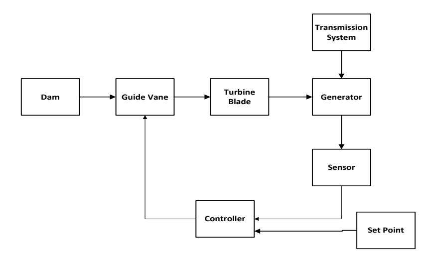
Figure 1 Block diagram of Saguling GBU control system
3 Identification System
3.1 Identification Fundamentals
Identification is a process to find model of a process or system based on experimental data provided. With such model, the characteristics of the system can be known and analyzed [3]. Figure 2 shows the identification steps.
Identification process first begin by designing an appropriate experiment which later sets of data will be aqcuisited from the experiment. The data obtained from variables entering the process and variables leaving the process. The next step is to choose the model structure, including the order of the system and choosing the estimation parameter method. Afterwards, the model should be validated.
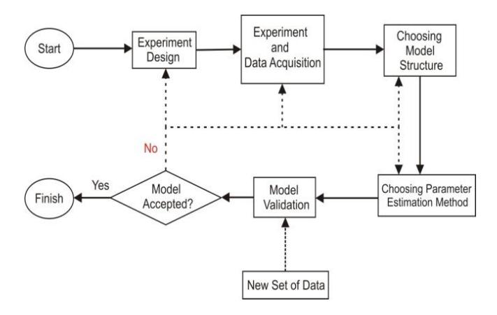
Figure 2 Identification steps
Turbine system was choosed because in startup condition, the process was focused in controlling the turbine angular speed. Figure 3 illustrate the relation between the input variable, the process and the output variable.
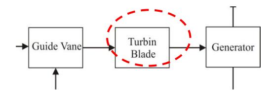
Figure 3 Turbine system
3.2 Neural Network
Neural network is a system which modeled human nerves system as a continuous nonlinear dynamic system. This network has nodes analogues with neuron in brain. Mathematical processes used in this network are also an approach to the way how brain works and also has the ability to learn from experience. Figure 4 illustrate the structure of neural network,
Figure 4 General neural network structure
A simple neural network structure can be expressed in,
\[y = f\left(\sum_{i=1}^{n} W_i U_i + b\right) \tag{1}\]
\(W_{1}\), \(W_{2}\), ....\(W_{n}\) and \(W_{b}\) are neural network weighthing parameters. These values will be evaluated in each iteration process. \(U_{1}\), \(U_{2}\), ... \(U_{n}\) are neural network inputs. Each one of them will be multiplied with weight W accordingly, which in turn will be summed and calculated with an activation function F. In result, the output Y will be known.
3.3 Backpropagation Algorithm
The main idea of this algorithm is to evaluate and modify the weights and bias in a way so the error value minimized. First step in this algorithm is choosing the cost function. Error is represented as the difference between desired output and output obtained from neural network learning. One of the cost functions used is the sum of quadratic error which defined in equation,
\[E = \frac{1}{2} \sum_{d} (O_{d} - y_{d})^{2}\] (2)
where \(O_d\) and \(y_d\) are the desired output and output obtained from neural network respectively. To minimize the cost function, the weights are evaluated with,
\[W(k+1) = W(k) - \eta \frac{\partial E}{\partial W}\] (3)
where W is weight, \(\eta\) is learning rate and E is cost function in error quadratic form. On outer layer, the gradient of cost function to weight is,
\[\frac{\partial E}{\partial W_{di}^{O}} = -\sum_{d} (O_{d} - y_{d}) \frac{\partial y_{d}}{\partial W_{di}^{O}}\] (4)
where \(W_{dj}^{\varrho}\) is the weight connecting the d- neuron from outer layer to j-neuron from hidden layer.
3.4 Identfication Using Neural Network
System was identified with previous acquisited data in non real time condition. 2250 number of data were used as turbine input and output, while guide vane opening was the input variable and turbine angular speed as the output variable. Time sampling used was 0.1 seconds. Identification process was done using neural network. Assumed a first order system with time delay. Based on this apriori knowledge, a neural network structure can be formed to be identified.
Based on (1), Saguling turbine system model can be illustrated with Figure 5,
Figure 5 ADALINE structure
And in mathematical equation,
\[y(k) = -y(t-1)a_1 + u(t-1)b_1\] (5)
Due to delay time in system response, (5) become,
\[y(k+nk) = -y(k-1+nk)a_1 + u(k-1)b_1\] (6)
with nk is the delay time, which values nk = 4 seconds. Figure 4 shows the model obtained from identification process while Figure 6 shows validated model.
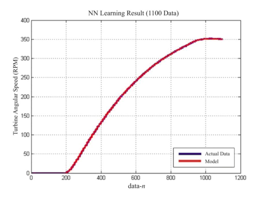
Figure 6 Model from NN learning and actual response
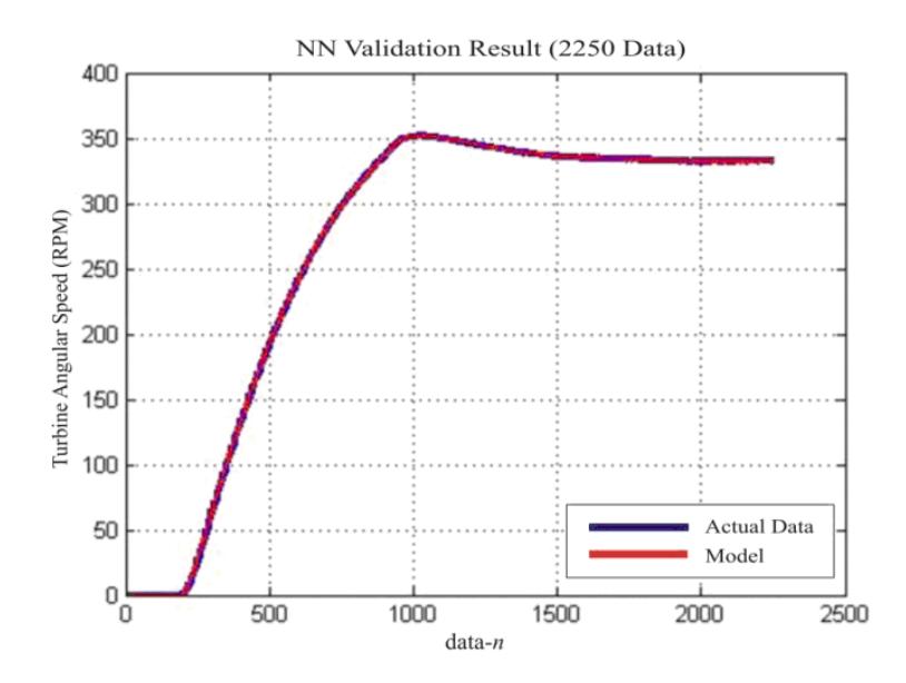
Figure 7 Model validation graphic
Root mean square error (RMSE) was used to analyze the closeness degree between identification result and the real value. RMSE defined by,
RMSE = \[\sqrt{\frac{\sum_{i=1}^{N} (y(\hat{i}) - \hat{y}(\hat{i}))^{2}}{N}}\] (7)
Table 1 shows the identification parameters result,
Table 1 Identification process parameters
| PARAMETER | Value |
|---|---|
| Data used for learning | 1100 |
| Data used for validation | 2250 |
| Learning Rate | 10.5 x 10⁻⁷ |
| Epoch | 1500 |
| RMSE from learning | 1.72 |
| RMSE from validation | 0.89 |
RMSE parameter in Table I shows the error value for each tracing point obtained between the model and the actual data. Saguling GBU can tolerate error value to 2 % which equals to range of response the systems can handle, that is 326.4 RPM to 339.66 RPM. From validation result, the system response vary from 332.11 RPM to 333.89 RPM, which means the error range still tolerable. Therefore, the model can be used to represent the process dynamics of the system.
The transfer function obtained from identification is.
\[H(z) = \frac{0.02847z^2 - 0.1137z + 0.881}{z^2 - 1.995z + 0.9949}\](8)
Information about delay time was already included in above equation. To design the controller, the model above should be multiplied with the actuator transfer function which was already known. Below equation is the actuator transfer function[6],
\[G(z) = \frac{0.003221}{z - 0.9968} \tag{9}\]
Thus, the whole process and the actuator transfer function become,
\[P(z) = G(z) \cdot H(z) = \frac{9.16 \times 10^{-5} z^2 - 3.66 \times 10^{-4} z + 2.83 \times 10^{-4}}{z^3 - 2.992z^2 + 2.983z - 0.9917}\](10)
4 Cotroller Design
4.1 Model Predictive Control (MPC)
MPC is a control strategy which designed based on model of certain processes. The model is used to calculate a set of future prediction output based on set of control signals given to the model. By using an optimization algorithm to minimize MPC cost function, a set of control signal can be obtained. Thus, controler performance really depends on the availability of a good model [4].
Model used in MPC in descrete state-space form can be represented as,
\[x(k+1) = A_d x(k) + B_d u(k)\] (11)
\[y(k) = C_d x(k) \tag{12}\]
\[z(k) = C_{z}x(k) \tag{13}\]
x(k) is state of the system, \(A_d\), \(B_d\) are output matrices, \(C_d\) and \(C_z\) is observable and controllable output matrice of the system respectively. Furthermore, prediction output can be obtained by iterating a model defined by,
\[\hat{z}(k+i|k) = C_z \hat{x}(k+i|k)\] \[= C_z A_d^i x + \sum_{j=1}^i C_z A_d^{j-1} B_d \hat{u}(k+i-j|k)\] (14)
Output prediction for the next k+j step, where state of the system on step k assumed to be known, can be recursively done and represented in matrice form.
\[\begin{bmatrix} \hat{z}(k+1|k) \\ \hat{z}(k+2|k) \\ \vdots \\ \hat{z}(k+H_{v}|k) \end{bmatrix} = \begin{bmatrix} C_{x}A_{d} \\ C_{x}A_{d}^{2} \\ \vdots \\ C_{x}A_{d}^{H_{v}} \end{bmatrix} \times (k) + \begin{bmatrix} C_{x}B_{d} \\ C_{x}A_{d}B_{d} + C_{x}B_{d} \\ \vdots \\ \sum_{i=0}^{H_{v}^{-2}} C_{x}A_{d}^{i}B_{d} \end{bmatrix} u(k-1)\] \[+ \begin{bmatrix} C_{x}B_{d} & \cdots & 0 \\ C_{x}A_{d}B_{d} + C_{x}B_{d} & \cdots & 0 \\ C_{x}A_{d}B_{d} + C_{x}B_{d} & \cdots & 0 \\ \vdots & \ddots & \vdots \\ \sum_{i=0}^{H_{v}^{-2}} C_{x}A_{d}^{i}B_{d} & \cdots & C_{x}B_{d} \end{bmatrix} \Delta \hat{u}(k+1|k)\] \[\vdots \\ \Delta \hat{u}(k+H_{v}-1|k)\]
With \(\Delta \hat{u}(k+i|k)\) is incremental input, which is \(\Delta \hat{u}(k+i|k) = \hat{u}(k+i|k) - \hat{u}(k+i-1|k)\). (15) can be simplified into [5],
\[\hat{Z}(k) = \underbrace{\psi \ x(k) + \gamma \ u(k-1)}_{past} + \underbrace{\Theta \Delta \hat{U}}_{future}\] (16)
The objective cost function is,
\[\text{[rumus tidak dapat ditampilkan dengan baik — lihat PDF asli]}\](17)
with Q and R are weighting matrices. The optimum of \(\Delta \hat{u}\) can be obtained by finding the gradient equals to zero of \(J_{MPC}\).
4.2 System Constraints
In practices, all processes have their constraints, such as input constraints, output constraints, incremental input constraints and state-space constraints. These constraints can exist in form physical constraints, like actuator limit.
The constraints can be expressed in form,
\[u_{\min} \leq \hat{u}(k+i \mid k) \leq u_{\max}\] \[\Delta u_{\min} \leq \Delta \hat{u}(k+i \mid k) \leq \Delta u_{\max}\] \[y_{\min} \leq \hat{y}(k+i \mid k) \leq y_{\max}\] \[x_{\min} \leq \hat{x}(k+i \mid k) \leq x_{\max}\] (18)
with \(u_{min}\), \(u_{max}\), \(y_{min}\), \(y_{max}\), \(x_{min}\) and \(x_{max}\) are minimum and maximum input, output and state constraints respectively.
4.3 Simulation
Due to the necessity of MPC for a discrete model, (10) was discretized so it changed into.
\[P(z) = \frac{9.16 \times 10^{-5} z^2 - 0.0003663z + 0.0002837}{z^3 - 2.992z^2 + 2.983z - 0.9917}\] (19)
Then (19) was transformed into state-space form so the value of each parameters in (11). (12) and (13) can be found, there are:
1. \[A = \begin{bmatrix} 2.992 & -1.492 & 0.4959 \\ 2 & 0 & 0 \\ 0 & 1 & 0 \end{bmatrix}\]
\[\mathbf{2.} \quad \mathbf{B} = \begin{bmatrix} 0.01563 \\ 0 \\ 0 \end{bmatrix}\]
3. \(C = \begin{bmatrix} 0.005868 & -0.01172 & 0.00908 \end{bmatrix}\)
4. \[D = [0]\]
The next step was to apply the parameters into MPC algorithm. MPC was then tuned to obtain the desired transient response. The tuning was limited only on weight R because manipulating Q gave no significant effect. The tuning parameters used in this simulation were.
- 1. Maximum Horizon = 10
- 2. Control Horizon = 3
- 3. Minimum Input Constraint = -10 V
- 4. Maximum Input Constraint = 10 V
- 5. Weight Q = 40 X 40 Identity matrice
Weight R was the parameter tuned to find the desired response. It is a 3 X 3 diagonal matrice which valued R = 0.01, R = 0.1 and R = 1.0 respectively. Figure 8 and Figure 9 shows the response and control signal comparation between manual control and system with MPC included as controller.
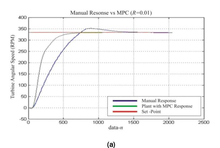
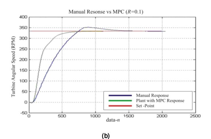
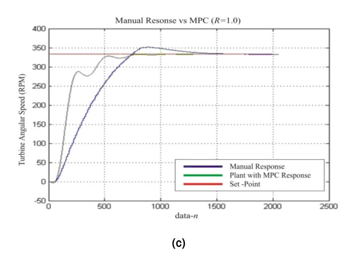
Figure 8 Comparation between manual vs system with MPC response with (a) R = 0.01, (b) R = 0.1, and (c) R = 1.0
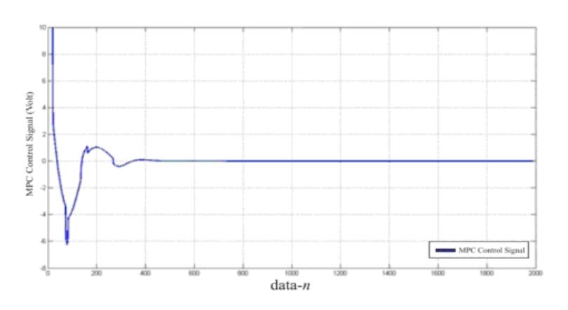
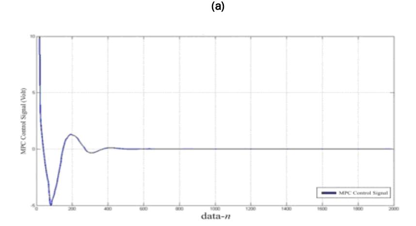
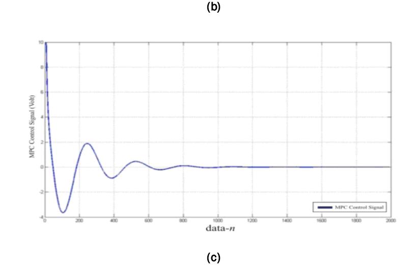
Figure 9 MPC control signal with (a) R = 0.01, (b) R = 0.1, and (c) R = 1.0
Table 2 shows the simulation result,
Table 2 System performance comparation with different weighting
| R | Performance Criterion | |
|---|---|---|
| Settling Time (Sec) | Maximum Overshoot | |
| 0.01 | 55.6 | None |
| 0.1 | 58.1 | None |
| 1 | 70.1 | None |
As can be seen in Figure 8, system response with MPC was faster compare to manual system. And it can be seen from Table II that settling time for MPC (55.6 sec, 58.1 sec and 70.1 sec) was faster than manual control (120 sec). As R smaller, the response became faster yet the signal control became more fluctuative, which can be seen in Figure 9. For mechanical system like turbine, an extreme fluctuation of control signals is undesirable due to actuator limitation. Therefore an appropriate value for R should be chosen carefully. In this experiment, the appropriate R would be 0.01. The control signal was qualitatively smooth enough and there were no overshoot.
5 Summary
From the simulation, a SISO turbine -generator system in Saguling GBU can be modeled, although there were many simplifications during identification process. The RMSE in identification process found to be 0.89, which is good enough to decide that the model accurately represent the real process. The model obtained was good enough to be used in simulation. Settling time criterion for system with MPC controller found to be 58.1 seconds, faster than using manual controller which is 120 seconds. In addition, system with MPC controller can eliminate the overshoot.
6 References
- [1] Anonymous, Deskripsi Indonesia Power UBP Saguling, Februari 2009, www.indonesiapower.co.id
- [2] Zuhal. Dasar Tenaga Listrik, Penerbit ITB, Bandung, 1991.
- [3] Soderstrom, Torsten and Stoica, Peter. System Identification. Marylands Avenue : Prentice Hall International (UK) Ltd, 1989.
- [4] Maciejowski, J. M., Predictive Control with Constraints, England: Prentice Hall, 2000.
- [5] Ling, K. V., "Introduction to Model Predictive Control," course notes, Bandung Institute of Technology, May 2008.
- [6] Manual Handbook Sistem Governor UBP Mrica, HPC 610 Water Turbine Governor, Asea Generation, 1985.