
1 Introduction and Objectives
One common goal in industrial chemical process designs is to achieve a specified product quality in feasible and profitable manners, despite the presence of feed fluctuations and other disturbances. One approach to accomplish such design is by formulating the simultaneous process and controller structure optimization as a mathematical programming problem, then subsequently utilizing a suitable computational algorithm to solve the problem.
The Dynamic Operability Framework is an optimization algorithm dedicated for such purpose. The framework formulates the process control design as a dynamic Mixed Integer Nonlinear Programming (MINLP) problem. The information processed by the framework consists of an objective (typically profit or operational costs), a set of Differential Algebraic Equations representing the process dynamics, a set of binary equations representing possible process control structures and interaction rules, a set of allowable ranges for operational conditions and a set of disturbance ranges.
This information is processed through two layers of computation. The outer layer optimization selects the structure and parameters of the process units and controllers. The inner level tests the controllability and feasibility of the process dynamics subject to a known range of disturbances over a given period of time. The framework iterates between these levels to generate the optimum solution.
The size of the problem is typically large. The computational complexities, i.e. requirement of CPU time, as well as Random Access Memory (RAM), may grow with the number of optimization variables. These aspects should be considered seriously in handling industrial cases that typically involves hundreds of dynamic variables.
In order to address such problem, this research investigates the computational tractability and optimality of the Dynamic Operability Framework. The results is the computational cost of a process design, based on the information supplied to the framework, such as the number of process parameters, dynamic variables, operational rules and constraints. The cost analysis is the basis to determine the computational requirement and processing time to produce an optimum process design through the framework. These will be especially useful to estimate the cost of a process design, the cost of further modification to the framework, as well as the benefit in distributing of the computational tasks in a number of parallel computers.
2 Process Synthesis Problem
Due to inherent nonlinearities, chemical processes present varying dynamic characteristics over different operating conditions and different structures. Consequently, a certain dynamic and economic performances can only be achieved by optimizing the process and controller structures, in addition to optimizing the controller parameters. At this point, the difficulty arises due to strong interaction between both aspects, as these cannot be isolated and optimized separately. This interaction between structure and parameter in process design, in pursuing the economic and control objectives, is best addressed within process synthesis problems.
The synthesis problem is to select the optimum process structure, as well as its design parameters. It involves rigorous analysis of the existence and interconnection of unit operations, as well as the sizes and parameters of the components. The former clearly implies making discrete decisions, while the latter implies making a choice from among a continuous space. The analysis ultimately determines the quality of process controllability and profitability in presence of disturbances and uncertainties.
Over the last three decades, process synthesis problems have been investigated using the heuristic, the physical insights, and the mathematical programming approaches. The physical insights yield in many essential design procedures and guidelines. Nevertheless, the developments of automated synthesis procedures are mostly based either on the knowledge based heuristic, or on mathematical programming approach.
The latter approach translates the process synthesis problem into the process control parameters and structures specification problem to satisfy the controllability and profitability objectives. These objectives are the consequence of two distinctive decisions. The first decision is the operational parameters, for instance, the size and operating conditions of the unit operations. These are represented by continuous values. The second decision is structure; i.e. the existence of a unit, a stream flow rate, or an interconnection between process units. These may involve yes-no, if-then and other logic decisions, as well as selection of distinct operational ranges. Hence, these values are discrete. The consideration of these decisions gives rise to Mixed Integer Nonlinear Programming (MINLP) problems.
3 The Dynamic Operability Framework
The Dynamic Operability Framework (DOF) is a mathematical programming algorithm developed to select the best configuration from a given set of possib le process and controller structures (a superstructure). The goal is to find the process structure and parameters that produces the optimum value of process objective (i.e. profit or target quality) and keeps all dynamic responses within the desired output space (completely
feasible). The selection is made subject to a set of expected disturbances, operational constraints and operational logics. The general formulation of the Dynamic Operability Framework to solve the mentioned design problem is given below.
\[\begin{split} & \underset{\overline{z}}{\min} \Phi(\overline{z}, \theta^{N}(t), x(t), \dot{x}(t), u(t), w(t), p, t)_{t=\overline{t}} \\ & s.t. \quad h_{i}(\overline{z}, \theta^{k}(t), x(t), \dot{x}(t), u(t), w(t), p, t) = 0 \\ & g_{j}(\overline{z}, \theta^{k}(t), x(t), \dot{x}(t), u(t), w(t), p, t) \leq 0 \\ & g_{jd}(y) \leq 0 \\ & F - OCI = \frac{\max_{\theta} AOS_{\theta}(\overline{w}(t))_{t_{0} \leq t \leq t_{f}} \cap DOS(\overline{w})}{DOS(\overline{w})} = 1 \\ & \overline{z} \in \{z, y, x_{ss}, u_{ss}, w_{ss}\} \\ & z \in Z = \{z : z^{1} \leq z \leq z^{u}\} \\ & \theta^{N} \in \theta^{k} \in EDS = \{\theta : \theta^{1} \leq \theta \leq \theta^{u}\} \\ & \overline{w}(t) \in w(t) \in \{x(t), u(t), w(t)\} \\ & x_{ss} = x(t = t_{0}) \\ & w_{ss} = w(t = t_{0}) \\ & t \in \{t : t_{0} \leq t \leq t_{f}\} \end{split}\]
Here, \(\overline{z}\) is the augmented vector of continuous and binary design variables z and y, and the initial conditions of state, manipulated, and output variables \(x_{ss}\), \(u_{ss}\) and \(w_{ss}\) respectively. The vector p contains the process parameters, and \(\theta_e\) contains the sampled disturbance profiles within the Expected Disturbance Space (EDS). The process model is represented by a set of differential algebraic equations \(h_i\). The time average of the objective function profile \(\Phi\) is optimized within an optimization window. The set \(g_j\) is the feasible design values for both plant and controller. The set \(g_{jd}\) is the subset of \(g_j\), containing the logic propositions to solve the mixed-integer problem related to the process control structure.
The Desired Output Space (DOS) defines the feasible dynamics of the output and measured variables in the augmented matrix \(\overline{w}\). The Achievable Output Space due to disturbances \((AOS_{\theta})\) is the set of output dynamics due to \(\theta_{e}\). The ratio between the size of \(DOS \cap AOS_{\theta}\) and the size of DOS is the controllability index, r-OCI. The external disturbances as well as process uncertainties are characterized as a set of step functions with uniformly distributed magnitudes in EDS.
Based on the above description, it is clear that DOF is a semi-infinite dynamic Mixed Integer Non-linear Programming (SIDMINLP) problem. The problem is solved in an iterative, two-layer dynamic optimization algorithm shown in Figure 1. The outer layer is a combined steady state and dynamic multi-period MINLP problem, that considers the regulatory process dynamics due to the critical disturbance and uncertainty combinations \(\theta^k\). At the initial outer level, \(\theta^k\) only consists of the nominal disturbances and uncertainties \(\theta^N\). The optimum solution \(\bar{z}^*\) found in the outer layer is sent to the inner layer, which performs the feasibility test for the framework. This layer evaluates the process feasibility at \(\bar{z}^*\) and extracts the associated \(\theta^k\) from the convex hull of \(AOS_\theta\). The iteration terminates when the outer layer converges and the inner layer does not introduce any additional \(\theta^k\), and this typically happens in the second iteration.
The outer layer consists of MINLP problem. The discrete variables represent superstructure that leads to Integer Programming (IP) Problem. The process model and operational constraints on each structure introduce Nonlinear Programming (NLP) sub problems.
Branch and Bound (BB) algorithm has been modified to solve these combined problems effectively. The search starts by solving the NLP relaxation of the original problem, then using the solution as the bound of the problem. If the solutions of the discrete variables are all equal to the values defined at the discrete set, then the optimum solution is reached and the search is stopped. Otherwise, the search fixes all discrete variables to their respective closest discrete values. Any purely discrete equation within the MINLP formulation is enforced to eliminate infeasible nodes. For example, the constraint y1+y2 1 eliminates the node [0,0].
The feasible nodes are considered as NLP sub problems. If one sub problem converges and the solution is better than the existing bound, this becomes the new bound, otherwise the node is eliminated. All previously evaluated binary combinations are listed to avoid repeated search.
The inherent nonlinearities of process models and the solution of process dynamics in each NLP sub problem significantly contribute to the computational cost. This grows exponentially with the number of design variables as described in Problem Background.
3.1 The Computational Analysis of DOF
The MINLP nature of the DOF algorithm requires the solution of one Integer Problem (IP) on distributing layer and one NLP at each nodes of the IP. These have been known as NP-Hard problems in. However, it should be noted that NP-Hardness is a worst case condition. There are features that make the DOF algorithm viable, such as [4]:
- 1. The r-OCI test in the first inner layer uses the convex-hull of the process dynamics to determine all critically affecting disturbances k . The whole set of k is attended on the second outer layer, and typically no new disturbances detected by the subsequent inner layer. Therefore the algorithm is typically completed in two iterations.
- 2. The IP in the distributing layer is solved by the modified BB algorithm. The general BB complexity usually determined by the number of discrete variables. In the worst case of case of all 0/1 decisions, all nodes have to be checked, hence the complexity is O(2n). In DOF, the modified BB uses the pure logic proposition constraints to significantly eliminate infeasible nodes from the tree and reducing the computational complexity accordingly. For example, if only one of two equipments y1 and y2 is allowed to operate, then the associated logic propositions is y1+y2 = 1. Then the possible nodes in enumeration tree are {[0,1],[1,0]}, instead of all four possible binary combination of [y1,y2]. The use of this proposition reduces 50% of computation efforts.
- 3. At each feasible node in the distributing layer, one dynamic NLP sub problem is solved. Once first converging sub problem with an objective value is found, this becomes the upper bound for the next sub problem. If the new sub problem shows any sign of inferiority, i.e. whether not converging or converging to poorer, then the node is fathomed and the algorithm resumes the search at the other nodes
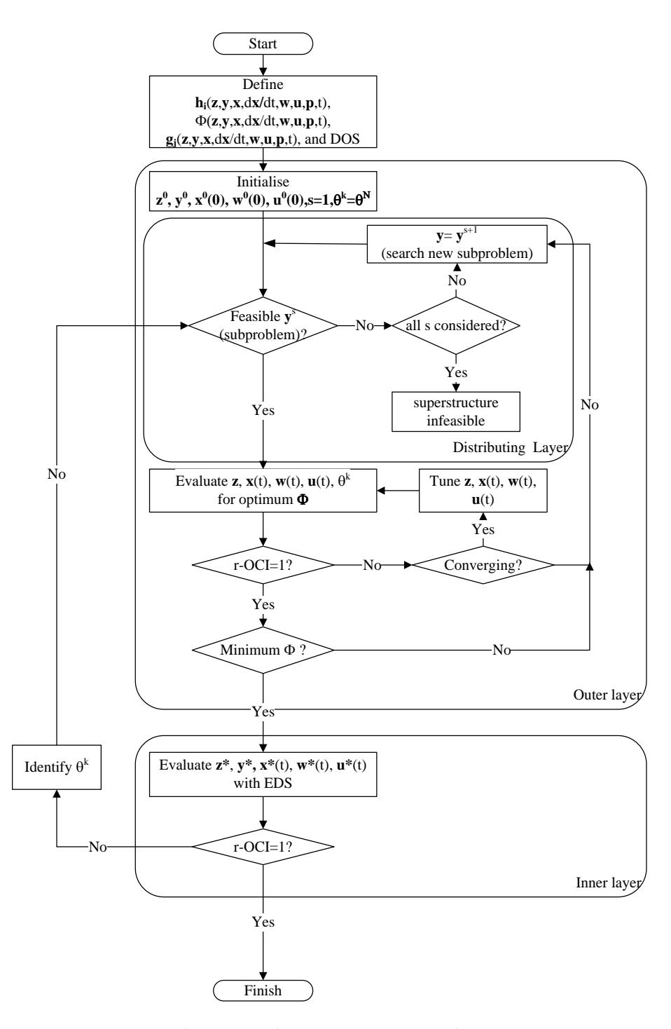
Figure 1 Algorithm of the dynamic operability framework
4 Computational Measures
To relate the computational costs of DOF problem, the following measures are employed: The size of the optimization problem specified by the number of continuous design variables nz, binary variables ny, and DAE describing the system i, operational constraints j and logic proposition jd, and samples of \(n\theta\). The contributions of these parameters to DOF complexity in relation to the algorithm depicted in Figure 1 are as follows:
- 1. The complexity of the NLP optimization problem in the outer level at the worst case is proportional to the number of continuous design variables nz.
- 2. The complexity of the modified Branch and Bound algorithm in the outer level at the worst case is exponential to the number of binary variables ny, i.e. 2ny. However, the number of logic propositions can reduce the complexity, although at the worst case, only 1 node is fathomed for each logic proposition. Hence at the worst case the complexity is 2ny-jd.
- 3. At the inner level, the complexity is proportional to the number of samples of \(\theta\) (n\(\theta\)) since all are required to determine the convex hull of the process dynamics. Incorporating all samples of \(\theta\) is essential to DOF, in order to anticipate the nonconvexities of the problem. The critically affecting disturbances \(\theta\)k found in this inner layer in the worst case is also proportional to n\(\theta\). If the first inner level declares all \(\theta\) as \(\theta\)k, then the second outer layer attends the whole set of\(\theta\). Consequently the second inner layer does not find a new \(\theta\)k. Therefore, even in the worst case, the algorithm concludes in two iterations.
- 4. The complexity of solving the process dynamic at every levels is proportional to the size of process model hi.
- 5. Since the complexity of NLP is NP-Hard, a worst case duration to solve the Sequential Quadratic Programming algorithm to solve one NLP node for one continuous design variables, TNLP is used to represent the NLP complexity. Similar term TDAE is used to represent the worst case time required to solve one DAE.
- 6. Based on the above contributions, the total complexity of DOF (CI) is as follows:
\[CI = 2 \times \left(T_{NLP} \times n_z \times (2^{n_y} - jd) + 1\right) \left(T_{DAE} \times n_\theta \times i\right) (2)\]
To obtain more specific information about the complexity of the optimization problem defined above, the reduction of DOF complexity due to the numbers of problem parameters is investigated for two case studies.
5 Case Studies
Two case studies of process and control structure selection of chemical process superstructures presented in the following sections. These cases a re:
- 1. Dual Continuous Stirred Tank Reactors (CSTR)
- 2. Five Effect Evaporator
5.1 The Dual CSTR
The objective of this case study is to select both process and controller structure to maximize the net profit of the two Continuous Stirred Tank Reactors (CSTR) system ([3]. The net profit is defined as the objective function as follows:
\[\Phi_{N} = 10(Q_{f1}C_{fN} + Q_{f2}C_{fN} - 0.3(Q_{f1} + Q_{f2})) - 0.01Cool_{1} - 0.1Cool_{2} - 0.1(Q_{f1} + Q_{f2})\] (3)
The dynamic variables are the product compositions C<sub>1</sub>, C<sub>2</sub> and temperatures T<sub>1</sub>, T<sub>2</sub>. The feasible operating conditions are defined by the temperatures T<sub>1</sub>, T<sub>2</sub>, the amount of heat transfer between coolant and reactor Cool<sub>1</sub>, Cool<sub>2</sub> and the final product composition Cp. The coolant flow rates mc1 and mc2 are manipulated variables that may control either T<sub>1</sub> or Cool<sub>1</sub> and T<sub>2</sub> or Cool<sub>2</sub>, respectively.
The problem is to decide the existence of the flow rates Qf<sub>1</sub>, Qf<sub>2</sub>, Q<sub>3</sub> and Q<sub>4</sub>. At least one of Qf<sub>1</sub> or Qf<sub>2</sub>, and one of Q<sub>3</sub> or Q<sub>4</sub> should exist, which leads to series, parallel, or combination process configuration. These decisions are facilitated by assigning four additional binary variables yp<sub>1</sub>, yp<sub>2</sub>, yp<sub>3</sub>, and yp<sub>4</sub> to the respective flow rates. Furthermore, the effect of reactor volumes V<sub>1</sub> and V<sub>2</sub> to both process and controller structures is evaluated. Therefore, the design variables are \(Qf_1\), \(Qf_2\), \(Q_3\), \(Q_4\), \(\alpha_1\), \(\alpha_2\), \(V_1\), \(V_2\), \(V_2\), \(V_2\), \(V_2\), \(V_2\), \(V_2\), \(V_3\), \(V_4\), \(V_4\), \(V_5\), \(V_4\), \(V_5\), \(V_5\), \(V_7\), \(V_8\), \(V_9\), \(V_9\), \(V_9\), \(V_9\), \(V_9\), \(V_9\), \(V_9\), \(V_9\), \(V_9\), \(V_9\), \(V_9\), \(V_9\), \(V_9\), \(V_9\), \(V_9\), \(V_9\), \(V_9\), \(V_9\), \(V_9\), \(V_9\), \(V_9\), \(V_9\), \(V_9\), \(V_9\), \(V_9\), \(V_9\), \(V_9\), \(V_9\), \(V_9\), \(V_9\), \(V_9\), \(V_9\), \(V_9\), \(V_9\), \(V_9\), \(V_9\), \(V_9\), \(V_9\), \(V_9\), \(V_9\), \(V_9\), \(V_9\), \(V_9\), \(V_9\), \(V_9\), \(V_9\), \(V_9\), \(V_9\), \(V_9\), \(V_9\), \(V_9\), \(V_9\), \(V_9\), \(V_9\), \(V_9\), \(V_9\), \(V_9\), \(V_9\), \(V_9\), \(V_9\), \(V_9\), \(V_9\), \(V_9\), \(V_9\), \(V_9\), \(V_9\), \(V_9\), \(V_9\), \(V_9\), \(V_9\), \(V_9\), \(V_9\), \(V_9\), \(V_9\), \(V_9\), \(V_9\), \(V_9\), \(V_9\), \(V_9\), \(V_9\), \(V_9\), \(V_9\), \(V_9\), \(V_9\), \(V_9\), \(V_9\), \(V_9\), \(V_9\), \(V_9\), \(V_9\), \(V_9\), \(V_9\), \(V_9\), \(V_9\), \(V_9\), \(V_9\), \(V_9\), \(V_9\), \(V_9\), \(V_9\), \(V_9\), \(V_9\), \(V_9\), \(V_9\), \(V_9\), \(V_9\), \(V_9\), \(V_9\), \(V_9\), \(V_9\), \(V_9\), \(V_9\), \(V_9\), \(V_9\), \(V_9\), \(V_9\), \(V_9\), \(V_9\), \(V_9\), \(V_9\), \(V_9\), \(V_9\), \(V_9\), \(V_9\), \(V_9\), \(V_9\), \(V_9\), \(V_9\), \(V_9\), \(V_9\), \(V_9\), \(V_9\), \(V_9\), \(V_9\), \(V_9\), \(V_9\), \(V_9\), \(V_9\), \(V_9\), \(V_9\), \(V_9\), \(V_9\), \(V_9\), \(V_9\), \(V_9\), \(V_9\), \(V_9\), \(V_9\), \(V_9\), \(V_9\), \(V_9\), \(V_9\), \(V_9\), \(V_9\), \(V_9\), \(V_9\), \(V_9\), \(V_9\), \(V_9\), \(V_9\), \(V_9\), \(V_9\), \(V_9\), \(V_9\), \(V_9\), \(V_9\), \(V_9\), \(V_9\), \(V_9\), \(V_9\), \(V_9\), \(V_9\), \(V_9\), \(V_9\), \(V_9\), \(V_9\), \(V_9\), \(V_9\), \(V_9\), \(V_9\), \(V_9\), \(V_9\), \(V_9\), \(V_9\), \(V_9\), \(V_9\), \(V_9\), \(V_9\), \(V_9\), \(V_9\), \(V_9\), \(V_9\), \(V_9\), \(V_9\), \(V_9\), \(V_9\), \(V_9\), \(V_9\), \(V_9\), \(V_9\), \(V_9\), \(V_9\), \(V_9\), \(V_9\), \(V_9\), \(V_9\), \(V_9\), \(V_9\), \(V_9\), \(V_9\), \(V_9\), \(V_9\), \(V_9\), \(V_9\), \(V_9\), \(V_9\), \(V_9\), \(V_9\), \(V_9\), \(V_9\), \(V_9\), \(V_9\), \(V_9\), \(V_9\), \(V_9\), \(V_9\), \(V_9\), \(V_9\), \(V_9\), \(V_9\), \(V_9\), \(V_9\), \(V_9\), \(V_9\), \(V_9\), \(V_9\), \(V_9\), \(V_9\), \(V_9\), \(V_9\), \(V_9\), \(V_9\), \(V_9\), \(V_9\), \(V_9\), \(V_9\), \(V_9\), \(V_9\), \(V_9\), \(V_9\), \(V_9\), \(V_9\), \(V_9\), \(V_9\), \(V_9\), \(V_9\), \(V_9\), \(V_9\), \(V_9\), \(V_9\), \(V_9\), \(V_9\), \(V_9\), \(V_9\), \(V_9\), \(V_9\), Vas the initial conditions of T<sub>1</sub>ss, T<sub>2</sub>ss, C<sub>1</sub>ss, C<sub>2</sub>ss, Cool<sub>1</sub>ss, and Cool<sub>2</sub>ss.
This superstructure is assessed in a closed-loop condition with a Proportional - Integral (PI) controller structure. The optimum parameters values are optimized further using the scaling factors \(\alpha_1\) and \(\alpha_2\). The binary assignments related to controller and process structure are given in Table 1 and Table 2 respectively.
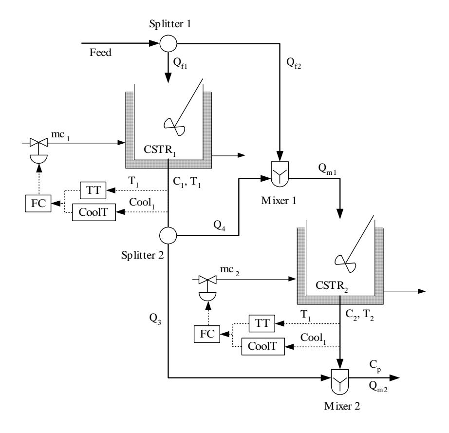
Figure 2 Dual CSTR problem
The superstructure model is as follows:
\[\text{[rumus tidak dapat ditampilkan dengan baik — lihat PDF asli]}\]
\[V_2 \frac{dC_2}{dt} = -k_0 e^{-Ec/RT_2} C_2 V_2 + Q_{ml} (C_{ml} - C_2)\]
\[V_2 \frac{dT_2}{dt} = D_h k_o e^{-Ec/RT_2} C_2 V_2 + Q_{ml} (T_{ml} - T_2) + Cool_2\]
\[\text{Cool}_2 = \frac{U_a m_{c2} cp}{U_a + m_{c2} cp} (T_{c2} - T_2)\]
\[Q_{m2} = Q_{ml} + Q_4 \quad C_p = \frac{(Q_4 C_1 + Q_{ml} C_2)}{Q_{m2}}\]
Table 1 Control parameters and logical assignments
| Control loop | Binary | Proportional | Reset | ||
|---|---|---|---|---|---|
| i | Control pair | Assignment | gain Ki | times \(\tau_l\) | |
| 11 | T1 - Mc1 | yc1 = 1 | -3.876 | 9.346 | |
| 12 | Cool1 - mc1. | yc1 = 0 | 3.79 | 6.135 | |
| 21 | T2 - mc2 | yc2 = 1 | -3.876 | 9.346 | |
| 22 | Cool2 - mc2. | yc2 = 0 | 3.79 | 6.135 | |
| int1 | T1 - mc2 | yc2 = 0 | 0.0013 | 1.5 | |
idx = controller parameter index
Table 2 Process structure and binary assignments
| Binary assignments | Decision | Binary assignments | Decision | |
|---|---|---|---|---|
| \(y_{p1} = 0\) | Qf1 off | yp1 = 1 | Qf1 on | |
| \(y_{p2} = 0\) | Qf2 off | \(y_{p2} = 1\) | Qf2 on | |
| \(y_{p3} = 0\) | Q3 off | \(y_{p3} = 1\) | Q3 on | |
| \(y_{p4} = 0\) | Q4 off | yp4 = 1 | Q4 on | |
The associated constraints for these design variables are as follows:
\[\begin{array}{lll} g_1: T_1 \leq 350 & g_2: T_2 \leq 350 \\ g_3: Cool_1 \leq 30 & g_4: Cool_2 \leq 20 \\ g_5: C_2 \leq 0.3 & g_6: Q_{f1} + Q_{f2} \leq 0.8 \\ g_7: Q_{f1} \geq 0.05y_{p1} & g_8: Q_{f1} \leq 0.8y_{p1} \\ g_9: Q_{f2} \geq 0.05y_{p2} & g_{10}: Q_{f2} \leq 0.8y_{p2} \\ g_{11}: Q_3 \geq 0.05y_{p3} & g_{12}: Q_3 \leq 0.8y_{p3} \\ g_{13}: Q_4 \geq 0.05y_{p4} & g_{14}: Q_4 \leq 0.8y_{p4} \\ g_{15}: 0 \leq \alpha_1 & g_{16}: \alpha_1 \leq 2 \\ g_{17}: 0 \leq \alpha_1 & g_{18}: \alpha_1 \leq 2 \\ g_{19}: V_1 \geq 4.5 & g_{20}: V_1 \leq 6 \\ g_{21}: V_2 \geq 4.5 & g_{22}: V_2 \leq 6 \\ g_{23}: y_{p1} + y_{p2} \geq 1 & g_{24}: y_{p3} + y_{p4} \geq 1 \end{array} \label{eq:g1}\]
All process dynamics are simulated over 100 seconds time horizon with 1-second intervals, and the outputs are Cool<sub>1</sub>, Cool<sub>2</sub>, mc<sub>1</sub>, mc<sub>2</sub>, and \(\Phi\)N; in addition to the state variables T<sub>1</sub>, T<sub>2</sub>, C<sub>1</sub>, C<sub>2</sub>, I<sub>11</sub>, I<sub>12</sub>, I<sub>21</sub>, and I<sub>22</sub>. The constraints g<sub>7</sub>-g<sub>14</sub> relates the binary decisions to the flow-rate existence. These relationships guarantee the amounts of flow-rate if yp=1, and none otherwise. At least one of Qf<sub>1</sub> or Qf<sub>2</sub> and one of Q<sub>3</sub> or Q<sub>4</sub> should exist, and these are represented by \(g_{23}\)-\(g_{24}\), which are evaluated in the integer feasibility test. The combination of the constraints \(g_{23}\)-\(g_{24}\) and the binary variables give rise to a 36 nodes enumeration tree at the dynamic MINLP problem.
5.2 The Five-Effect Evaporator
The five-effect evaporator superstructure is shown in Figure 3. The evaporator consists of one falling film, three counter-current forced circulation and one super-concentrator units. The controlled variables are the liquor levels hP1-5, the product density \(\rho\)P5 and the product temperature TP5. The candidates of manipulated variables are the product flow rates QP1-5, the live steam MS3-5, and the vaporization rate in the final stage MV5. The energy transfers involve the live steam MS3-5, the vapor MV1-5, the condensates MC1-5, and the recycle streams MHF1-4. The disturbances are the fluctuations of the feed flow rate QF, the feed temperature TF and the cooling water temperature TCW, which have been sampled and held every 30 minutes. The interaction between these variables gives rise of 32 Differential Algebraic Equations for each tank that develop the process model.
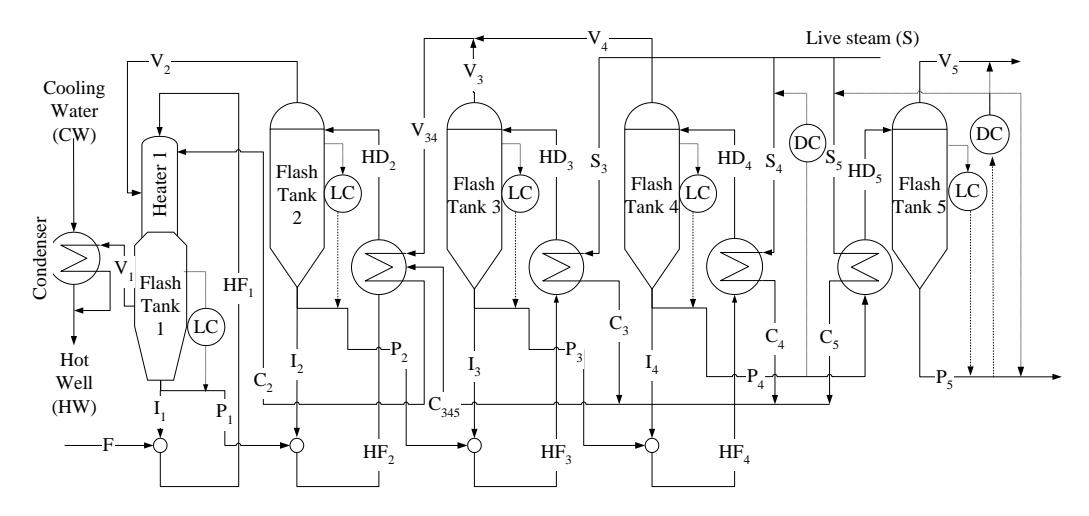
Figure 3 Five effect evaporator
The superstructure facilitates the distribution of live steam to the last three stages, the mixing of vapor from stage 3 - 4, and the alternative matching between measurements and manipulated variables. The process structure is associated with the binary decision variables for the distribution of live steams, yP3-5. The variables determine the operation of three, four or five-effect modes to achieve the target density. At least one of the stages 3 or 4 has to be operated; and if both are, the vapor from both stages is mixed.
Table 3 Control loops and parameters
| Dec- ision | Out- put | In- put | Kc | τ (hr) | Note | Dec- ision | Out- put | Input | Kc | τ(hr) | Note |
|---|---|---|---|---|---|---|---|---|---|---|---|
| - | hP1-4 | QP1-4 | 25 | always active | Ус4 | ρр5 | QP5 | 50 | 0.05 | PI control | |
| Ус1 | hP1-4 | QP1-4 | 1 | I control | УС5 | ρч | MS34 | -30 | 2 | ||
| yc1 | hP5 | QP5 | 1 | УС6 | ρг | MS5 | 100 | 1 | |||
| Ус1 | hP5 | MV5 | 0.5 | УС7 | ρр5 | MV5 | -100 | 1 | |||
| yc2 | hP5 | QP5 | 25 | P control | Ус8 | TP5 | MS5 | -0.2 | 1 | ||
| Усз | hP5 | MV5 | 20 | УС9 | TP5 | MV5 | -0.01 | 0.1 |
The controller structure is represented by the binary decision variables yC1-9, which activate the control-loops properties of a multi-loop Proportional-Integral (PI) feedback control scheme as summarized in
Table 3. The gains Kc1-9 and the reset times 1-9 are pre-designed for stability. The binary variables are constrained such that each manipulated and controlled variable can only be used once within the control scheme, and only activated if the associated process structure is active. For instance, hP5-QP5 can only be activated if stage 5 is active. The parameters of active control loops can be tuned further with the scaling variables 0 1-9 2. The process optimization problem is associated with the maximization of the profit subject to the feasible process dynamics, as well as the logics of interconnection between the process and controllers.
6 Results and Discussions
The CSTR problems parameters include 14 continuous design variables, 6 binary design variables, 22 differential algebraic equations, 22 constraints and 2 logic propositions. Meanwhile, the Evaporator problems parameters include 40 continuous design variables, 9 binary design variables, 160 differential algebraic equations, 22 constraints and 2 logic propositions. The worst case durations of operation are measured as the maximum duration for both cases in a Pentium IV Personal Computer, 2.4 GHz, 512 MB RAM with 0.05% confidence. Based on these measurements, TNLP and TDAE are 0.5 seconds and 0.2 seconds respectively. Based on equation (2), the complexity indices for these cases, in comparison to the duration of experimental optimization results are:
Table 4 Comparison between computational index and experimental duration
| Case | CI (in seconds) | Experimental duration (in seconds) | |||
|---|---|---|---|---|---|
| Dual CSTR | 797.5 | 301.2 | |||
| Evaporator | 199484.91 | 83537.4 | |||
Compared to the empirical results, the theoretical worst-case computational indices are twofold of the experimental durations. These show that the MINLP problems are solved efficiently in comparison to the worst case complexity. In these cases, the logic propositions provide the most contribution to fathom the structural nodes of the modified Branch and Bound algorithm. At cases, the proportionality and the gap between CI and the experimental duration gives a promising uses as the measure of computational efforts of process control design based on mathematical programming approach and further study of assessing the efficiency of optimization algorithms.
7 Conclusion
The worst case complexity of Dynamic Operability Framework has been formulated based on the size of the optimization problem specified by the number of continuous design variables nz , binary variables ny, and DAE describing the system i, operational constraints j and logic proposition jd, and samples of n. The resulting complexity indices are relatively proportional to the experimental duration and the gaps provide a promising use as the quantification of the efficiency of the algorithm.
8 References
- [1] Blondel, V. D., Tsitsiklis, J. N., Automatica, 1999(35): 479 489.
- [2] Blondel, V. D., Tsitsiklis, J. N., Automatica, 2000(36): 1249 1274.
- [3] Ekawati, E. and Bahri, P. A. Journal of Process Control, 2003(13-8): 717 - 727.
- [4] Ekawati E. and Bahri, P.A. CHEMECA 2004, 2004.
- [5] Floudas, A., Mixed Integer Nonlinear Programming, 1995.
- [6] Goyal, V., Ierapetritou, M. G., Computers and Chemical Engineering, 2004
- [7] Nishida, N., Stephanopoulos, G. and Westerberg, A. W., AIChE Journal, 1981(27): 321 351.
- [8] Papadimitriou, C. and Steiglitz, K., Combinatorial Optimization; Algorithms and Complexity, 1982
- [9] Till, J., Engell, S., and Panek, S., Stursberg, O, IFAC-Conference Analysis and Design of Hybrid Systems, 2003
- [10]Wang, L., Journal of Systems Science and Complexity, 2001(14-1)
- [11]Wolff, E. A., Skogestad, S., Hovd, M. and Mathisen, K. W., IFAC workshop on Interactions between Process Design and Process Control, 1992