
1 Introduction
The industries produce waste heat in a varied range of temperature. Generally, the waste heat produced is directly exempted to the environment without any further utilization. This causes a few problems; the increase of heat pollution being one of it. Despite its impact to the environment, the waste heat ejected still contains significant amount of useful heat that can be utilized to generate power [1]. In geothermal fields, the brine that has been used in the power plant will be injected back to the reservoir through the injection well [2]. A technology and an operational system that can effectively utilize the thermal energy from the brine before sending it back to the reservoir is of high importance. The number of production and injection wells needed can be reduced by effectively utilizing the thermal energy contained in the brine [3]. The brine that will be sent back to the reservoir through the injection well has a temperature of 150°C - 170°C or 423 K – 443 K. With that range of temperature, the brine still contains a significant amount of useful heat that may be considered. There are a few systems that can be implemented to recover this useful heat. An organic Rankine cycle is an adequate way to recover waste heat at the specified range of temperature [4]. The difference between a simple Rankine cycle and an organic Rankine cycle lies in the working fluid used in the cycle. Organic Rankine cycles utilizes working fluids of organic substances. Generally, organic fluids have lower boiling and critical points than water [5]. Typically, simple Rankine cycles that use steam as the working fluid are suitable for utilization of high-grade waste heat. One of the important factors to be considered in an organic Rankine cycle system is the type of working fluid. The working fluids must be selected carefully as they hold an important role in the system efficiency, cycle operation and its impact to the environment. Apart from the working fluid, system configuration must also be taken into account. A program package was needed to simulate the processes in the cycle. It can be used for simulation study of the thermal efficiency and working effectiveness of the system before the system is implemented in real life.
2 Literature Review
A Rankine cycle consists of four processes in four different components [6], as illustrated in Fig. 1. The components involved in the power generation through Rankine cycle are condenser, pump, evaporator, and turbine.
Figure 1. Scheme of an organic Rankine cycle.
The process of compression takes place in pump and is done to increase the pressure of the working fluid. The ratio of the pressure of working fluid at pump outlet to the pressure of working fluid at pump inlet is called pressure ratio. The isentropic efficiency of pump is calculated with equation (1).
\[\eta_p = \frac{h_{3s} - h_2}{h_{3a} - h_2} \tag{1}\]
The power needed by pump to do compression is defined by equation (2).
\[\dot{W}_{p} = \dot{m}(h_{3s} - h_{2}) = \dot{m} \eta_{p} (h_{3a} - h_{1})\] (2)
Waste heat enters evaporator and transfers its heat to the working fluid. The working fluid's temperature rises and changes its state from saturated liquid to saturated vapor. In the case of superheating, the working fluid exits the evaporator as superheated vapor. The process of heat exchange is also done in condenser. The working fluid transfers its heat to the cooling fluid and changes its state from vapor to liquid. Both processes in evaporator and condenser are carried out at a constant pressure. The E-NTU method helps predict the performance of the heat exchanger. It is specifically used when only the inlet temperatures of the heat exchanger are defined. The rate of heat transfer from hot fluid to cold fluid is expressed by equation (3).
\[q = \varepsilon C_{\min} (T_{h,i} - T_{c,i}) = \varepsilon C_{\min} \Delta T_{\max}\] (3)
The ratio of the actual heat transfer rate to the maximum possible heat transfer rate is called effectiveness. Heat transfer is said to be maximum when the outlet temperature of the hot fluid reaches the inlet temperature of the cold fluid or the outlet temperature of cold fluid reaches the inlet temperature of the hot fluid. Assuming that the heat exchanger is a counter flow type, the energy balance of both fluids is calculated by equation (4).
\[q = C_b(T_{b,i} - T_{b,o}) = C_c(T_{c,o} - T_{c,i})\] (4)
Turbine lowers the pressure of working fluid through expansion. The expansion ratio shows the ratio between the pressure of working fluid at the turbine inlet and the pressure of working fluid at the turbine outlet. The isentropic efficiency of turbine is defined by equation (5).
\[\eta_p = \frac{h_4 - h_{1a}}{h_4 - h_{1s}} \tag{5}\]
Power generation, which serves as the main purpose of a Rankine cycle, is done in turbine. The amount of power produced by turbine is calculated as follows:
\[\dot{W}_{t} = \dot{m}(h_{A} - h_{1a}) = \dot{m} \, \eta_{t} (h_{A} - h_{1s}) \tag{6}\]
Based on the slope of the saturation curve in the T-s diagram, organic working fluids are divided into three categories [7]; dry, wet and isentropic fluids. Dry fluids have positive slopes while wet fluids have negative slopes. Isentropic fluids have nearly vertical slopes. Wet fluids with negative slopes often contain saturated liquid at the outlet of turbine. The presence of liquid is avoided as it causes damage to the turbine blades. On the other hand, dry and isentropic fluids exit the turbine as vapor so damage caused by liquid or droplets can be prevented. Because of this thermal property, dry and isentropic fluids are more suitable for organic Rankine cycle.
3 Methodology
3.1 Selection of working fluids
Some factors that must be taken into account when selecting working fluids for an organic Rankine cycle are the temperature of the heat source, the slopes of saturation curve in the T-s diagram, the value of ODP and GWP100. Fluids of dry and isentropic types are preferred because they exit the turbine as vapour. This way, damage of the turbine blades can be avoided. The heat source that will be used utilized has a temperature range of 150°C -170°C and a mass flow rate of 3.125 kg/s. The working fluids must be able to work under the assigned working conditions. In other words, they should have critical points around the temperature of the heat source. However, it should be noted that the fluids must not operate at a temperature above the critical points. ODP shows the ratio of ozone depletion caused by a substance of a certain mass to the ozone depletion caused by CFC-11 with an identical mass. The values of ODP and GWP100 are obtained from CoolProp, a database that covers thermal properties of 122 fluids. Through consideration of the aforementioned factors, it was found that the following working fluids shown in Table 1 are suitable for waste heat recovery from geothermal water at the specified temperature range.
Fluids Tcrit (°C) ODP GWP100 Slope R141b 204.5 0.11 725 (+) R601 196.7 0 < 20 (+) R601a 187.35 0 < 20 (+) R245ca 174 0 < 20 (+) R600 152.125 0 3 (+) R124 122.425 0.02 609 (+) R236ea 139.44 0 1200 (+) R245fa 154.01 0 1030 (+)
Table 1. Selected working fluids.
3.2 Design of program package
The program package was constructed with MATLAB with a license number of 920421 to simulate the processes in the system cycle of organic Rankine. It consists of three main components; graphical user interface, calculation program and output data. The graphical user interface was built upon the GUIDE feature that has been provided in MATLAB. Users will have to insert values of some parameters in the interface before the program can be operated. The interface is equipped with guidance that is aimed to help users in deciding the value of each parameter. It is also equipped with three push buttons; 'Simulasi', 'Simpan', and 'Atur ulang'. Before pushing the 'Simulasi' button, users have to make sure that each blank space has been filled. The 'Simpan' button enables users to save the result from calculation in an Excel file. The 'Atur ulang' button can be used once users want to reset the program and start setting up new values of the parameters. The calculation program was constructed as a script file in MATLAB and will process the values inserted by users in the graphical user interface. The result of calculation will be presented on a new window once the 'Simulasi' button is clicked. It comprises thermal properties of the working fluid, such as temperature, pressure, enthalpy and entropy at each point in the cycle. The phase of the working fluid is included in the same panel as other thermal properties. It also shows work needed by pump, work produced by turbine, and the amount of heat transferred in the heat exchangers.
4 Result and Discussion
4.1 Procedure of program package usage
Users will have to install MATLAB to operate the program package. CoolProp, coupled with MATLAB, is used to calculate the thermal properties of the fluids involved in the system cycle. Users will need to choose one of the eight working fluids that have been provided in the graphical user interface. The high and low temperature of the working fluid must be defined by users as well. The isentropic efficiency of turbine and pump are set to 0.85 by default. Users may change these values. However, it should be noted that the isentropic efficiency of both pump and turbine must be less than 1. If users insert values that deviate
from the guidance, a warning sign will appear and users will have to correct the previously inserted values.
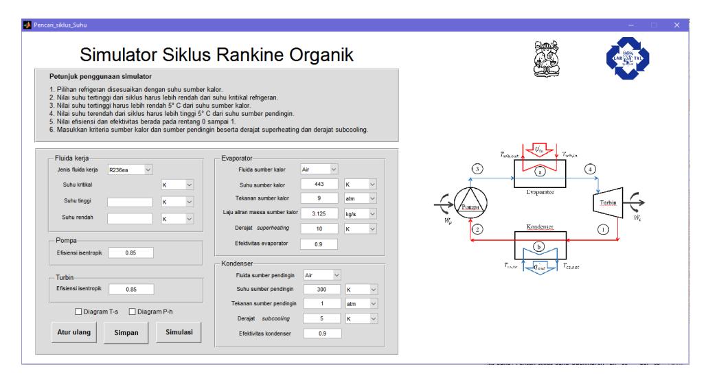
Figure 4. The interface of the program package.
4.2 Parametric analysis
Parametric analysis was conducted to see the effect of working fluid's high temperature and low temperature variations on thermal efficiency, power needed by pump, power produced by turbine, and the amount of heat transferred in the evaporator. R245fa was chosen as the working fluid. The waste heat had a temperature of 443 K at 0.9 MPa and was distributed with a mass flow of 3.125 kg/s. To avoid decomposition and deterioration, the working fluid's temperature must be lower than its critical temperature. The maximum temperature of the working fluid was set to 425 K with 10 degrees of superheating. The cooling fluid's temperature was assumed to be equal to ambient temperature. It was set to 300 K with a pressure of 0.1 MPa. The degree of subcooling was set to 5. Based on temperature approach, the temperature of the working fluid must be at least 5 K less than the temperature of cooling fluid. The pump and turbine were assumed to have an isentropic efficiency of 0.85. The effectivity of condenser and evaporator were assumed to be 0.9.
Simulations were done by varying the high and low temperature with an interval of 5 K in each variation. The lower limit of the low temperature was set to 305 K while the lower limit of the high temperature was set to 325 K. The minimum temperature difference of high and low temperature must be 20 K because of superheating and subcooling. ∆T denotes the difference between high temperature and low temperature. Fig. 5. shows that the increase in ∆T results in the increase in power needed by pump. The increase in ∆T generally means the increase in pressure difference between the pump outlet and the pump inlet. Consequently, the higher the pressure difference, the more power is needed by pump to compress the working fluid. The increase in ∆T would consequently increase the power generated by turbine, as shown in Fig. 6. The heat transfer processes in both evaporator and condenser are assumed to be conducted at a constant pressure. Hence, there are only two values of pressure in the system cycle. The working fluid is at a high pressure in evaporator and turbine. Once expanded, the working fluid flows at a low pressure to condenser and pump in sequence. In other words, the pressure ratio of pump equals to the expansion ratio of turbine. Therefore, the increase in ∆T will increase the pressure difference. Similarly, the increase in pressure difference will increase the power produced by turbine. The thermal efficiency of the cycle increases in accordance with the increase in ∆T, as shown in Fig. 6. It's been proven that the increase in ∆T will increase the power needed by pump and power produced by turbine. However, the increase in turbine power is higher than the increase in pump power. This will consequently increase the thermal efficiency of the cycle. The amount of heat transfer increases as ∆T increases. The higher ∆T means that more work is needed to rise the temperature of working fluid in the evaporator, as seen in Fig. 7.
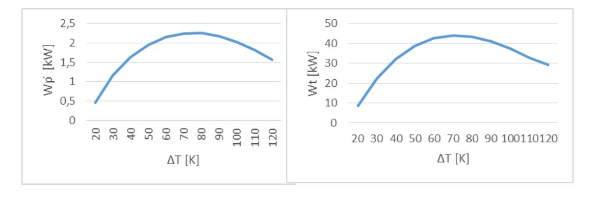
Fig. 2. Effect of ∆T on Wp. Fig. 3. Effect of ∆T on Wt .
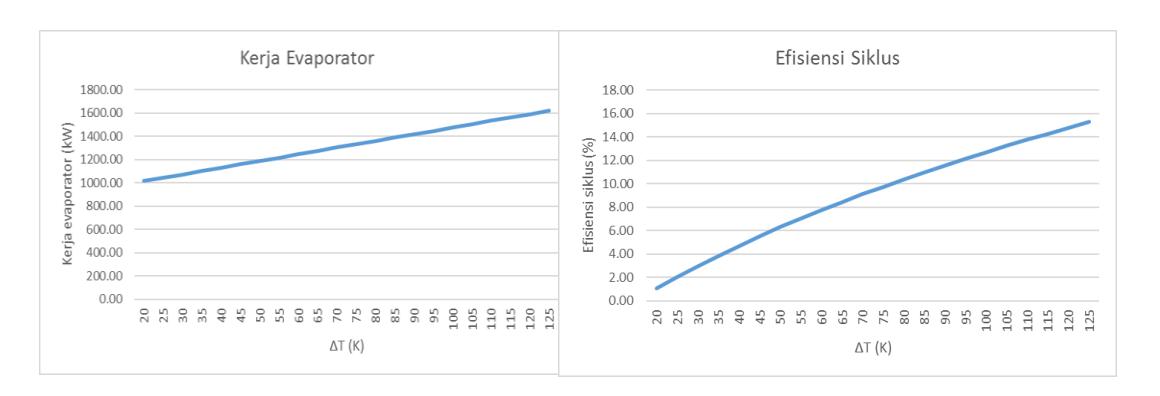
Fig. 4. Effect of ∆T on heat transfer in evaporator.
Fig. 5. Effect of ∆T on thermal efficiency.
4.3 Simulation results for different working fluids
Simulations were done using eight working fluids that have been chosen. The heat source temperature was varied to see the performance of each working fluid under different working conditions. The interval of each variation was set to 5 K, with 393 K as the lower limit and 463 K as the upper limit of the heat source temperature. In each variation, R141b ranks as the working fluid that gives the highest thermal efficiency with an average of 15.9%. N-pentane gives the second highest thermal efficiency with an average of 14.63%.
For heat source with a temperature of 448 K, R245ca and isopentane give the third and fourth highest thermal efficiency, respectively. However, for heat source at 453 K, isopentane gives higher thermal efficiency than R245ca. This is due to the different high temperature of R245ca and isopentane when the heat source temperature is set to 453 K. For heat source temperature of 448 K, both R245ca and isopentane have a high temperature of 443 K. The value 443 K was chosen based on the rule that the minimum temperature difference in a heat exchanger must be at least 5 degrees. On the other hand, when the heat source was set to 453 K, the high temperature of R245ca was set to 443 K due to the limitation of critical temperature. The critical temperature of R245ca is 447.57 K and this means that the high temperature must be set lower than the critical temperature. Since the critical temperature of n-pentane is higher, it was possible to set its high temperature to 448 K.
5 Conclusion
A simulator package that consists of graphical user interface, calculation program and output data was constructed using MATLAB that has been coupled with CoolProp. Using the simulator, parametric analysis was conducted to see the effect of system cycle's different working conditions on four parameters; thermal efficiency, power generated by turbine, power needed by pump. It was found that with a higher value of ∆T, the thermal efficiency increases. The similar response was found in power generated by turbine and power needed by pump.
6 Reference
- [1] Khennich, M. dan N. Galanis, "Optimal design of ORC systems with a low-temperature heat source," Entropy, pp. 370-389, 2012.
- [2] Wei, D., X. Lu, Z. Lu dan J. Gu, "Performance analysis and optimization of organic Rankine cycle (ORC) for waste heat recovery," Energy Conversion and Management, pp. 1113-1119, 2007.
- [3] …,"Office of Energy Efficiency and Renewable Energy," [Online]. Available: http://energy.gov/eere/geothermal/how-geothermal-power-plant-works-simple. [Accessed 23 August 2016].
- [4] Eliasson, E. T., S. Thorhallsson and B. Steingrimsson, "Geothermal power plants," in Short Course on Geothermal Drilling, Resource Development and Power Plants, Santa Tecla, 2011.
- [5] Cengel Y. A. dan M. A. Boles, Thermodynamics: an engineering approach, McGraw Hill, 2006.
- [6] Hettiarachchi, H. D. M., M. Golubovic, W. M. Worek dan Y. Ikegami, "Optimum design criteria for an organic Rankine cycle using low-temperature geothermal heat sources," Energy, pp. 1698-1706, 2007.
- [7] Saleh, B., G. Koglbauer, M. Wendland dan J. Fischer, "Working fluids for lowtemperature organic Rankine cycles," Energy, pp. 1210-1221, 2007.