1 Introduction

Research on the platooning system has been widely publicized and attracted attention from academics and industry. This is because such a system significantly impacts the highway's field of transportation [1], [2]. This platooning system provides an innovative idea about the automated way of driving a group of vehicles on the highway forming a lined formation, with the aim of fuel efficiency and accident reduction [3], [4]. In a group of Nvehicles connected in a platoon formation, the front vehicle is called the leader, while all the vehicles behind it are called followers. This system consists of coordinated movements of a group of vehicles to reach a common destination. The vehicle platoon control is viewed from the perspective of network control. The platoon is divided into four components: node dynamics, information flow topology, distributed controllers, and geometry formation [3], [5]. With the Vehicle-to-Vehicle (V2V) communication, it is possible for vehicles running on the highway to exchange information and then form a platooning system, whereas mentioned before, the front vehicle acts as the leader and the vehicles behind it as followers. Vehicles outside the platoon can communicate and join the group as platoon members. Members can leave the platoon once they reach their destinations. As a result, platoon members will vary at any point in time depending on their destinations. The platoon leader would also vary; when the leader has reached the destination, the leader can ask the vehicle behind to take over the job as a leader in the platoon system. This system also allows drivers to take over braking when the distance in front of the vehicle is too close to avoid accidents [1].

The V2V Communication system is based on the international standard IEEE 802.11p, also known as Wireless LAN [9], [10], [11], which regulates wireless communication systems in a driving environment. The 802.11p Standardization, known as WAVE (Wireless Access in Vehicular Environments), produces a communication protocol that runs on the 5.9 GHz band called DSRC (Dedicated Short-Range Communication). This can be used exclusively for communication between vehicles (V2V Communication) or Vehicle-to-Infrastructure Communication (V2I), most seen in developed countries. This system aims to realize an application that can help improve security in the driving and traffic environment.

There are various types of information flow topology, namely predecessor following, bidirectional, predecessor following the leader, bidirectional leader, two-predecessor following, and two-predecessor following leader [2], [3], [4], [5], [8]. Information flow topology has an impact that significantly influences the behavior of a platoon.

The platooning system generally depends on several factors, for example, the quality of communication signals, infrastructure, and intervehicle communication. This paper does not discuss the communication system between vehicles because it is assumed that vehicles incorporated in this platoon formation are equipped with an electronic system in the form of distance and velocity sensors. This information can maintain the optimal distance between vehicles and keep vehicle velocity constant at a steady state. In this paper, a simulation of the platoon system is made using distance and speed information obtained from vehicle sensors using a serial PID controller using appropriate PID parameters to keep the distance between vehicles constant at a steady state.

ISSN: 2085-2517

2 Platooning System

Vehicle longitudinal dynamic behavior of the platoon system is written in a nonlinear model. The parameters used are drive line, brake system, air friction, coefficient of wheel friction, and gravity [2], [3], [4], [5]. Position and velocity are usually expressed as variables p(t) and v(t), regardless of initial conditions. Velocity is a derivative of position, while the acceleration is a derivative of velocity. Using a control system stability analysis, the platooning system's asymptotic stability and string stability can be obtained by determining the control parameters. The main idea of this paper is to find the appropriate PID control parameters to solve the vehicle longitudinal dynamic behavior problem so that the distance between vehicles is maintained as desired and the speed of each vehicle is the same in a steady state.

2.1 Single Vehicle Control

The dynamic model of a single vehicle is expressed using the general vehicle dynamic model in [1], as shown in Figure 1.

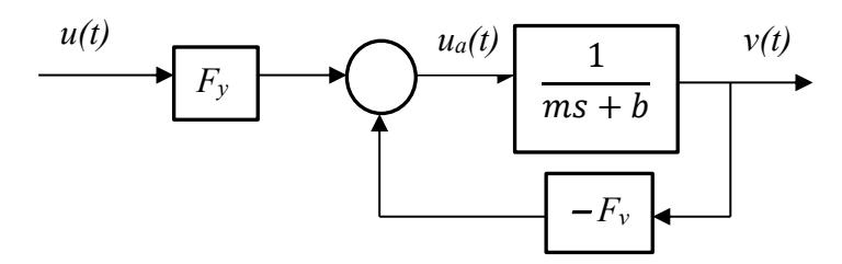
Figure 1. Vehicle's dynamic model [1]

The block diagram above can be represented in the equation below:

\[-F_{v}v(t) + F_{y}u(t) = m\dot{v}(t) + bv(t) + w(t)\] (1)

where \(F_y\) is feedforward gain and \(F_v\) is feedback gain of driving / braking signal; m is the vehicle's mass; b is tire/road rolling resistance; v(t) is the velocity of the vehicle; u(t) is the control signal and \(w(t) = cv^2(t)\). In an ideal condition, it is assumed that c=0; c is the aerodynamic drag coefficient. Hence the vehicle dynamic model (1) for the velocity variable can be expressed as [1]

\[\dot{v} = -\left(\frac{b}{m} + \frac{F_v}{m}\right)v(t) + \frac{F_y}{m}u(t) \tag{2}\]

The model above can then be illustrated by the block diagram as shown in Figure 2.

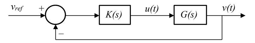
Figure 2. Vehicle's velocity control system [1]

K(s) is the PID controller, and G(s) is the vehicle's model, written in Laplace form:

\[K(s) = K_1 + \frac{K_2}{s} + K_3 s \tag{3}\]

\[G(s) = \frac{F_y}{ms + b + F_y} \tag{4}\] where \(K_1\) is the proportional gain, \(K_2\) is integral gain, and \(K_3\) is a derivative gain. Then we can write the open loop transfer function in standard form

\[G(s) = \frac{\omega_n^2}{s + 2\zeta\omega_n} \tag{5}\]

By comparing equations (4) and (5), the parameters \(\zeta\) and \(\omega_n\) can be expressed in the vehicle's parameters as follows [1]

\[\omega_n = \sqrt{\frac{F_y}{m}}\] and \(\zeta = \frac{b}{2\sqrt{mF_y}} + \frac{F_v}{2\sqrt{mF_y}}\)

The closed-loop transfer function of the vehicle velocity control system in Figure 2 can be written as

\[\frac{V(s)}{V_{ref}(s)} = \frac{K(s)G(s)}{1 + K(s)G(s)}\]

\[\frac{V(s)}{V_{ref(s)}} = \frac{K_3 \omega_n^2 s^2 + K_1 \omega_n^2 s + K_2 \omega_n^2}{(1 + K_3 \omega_n^2) s^2 + (2\zeta \omega_n + K_1 \omega_n^2) s + K_2 \omega_n^2}\](6)

This transfer function shows that system is internally stable, \(\frac{v}{v_{ref}}(s)=1\) for s=0, indicating that the error \(\left(v_{ref}(t)-v(t)\right)\to 0\) at \(t\to\infty\)

The position of vehicle y(t) moving straight is expressed with the integral of velocity v(t) so that the plant G(s) becomes:

\[P(s) = \frac{1}{s}G(s) = \frac{\omega_n^2}{s(s+2\zeta\omega_n)} \tag{7}\]

The reference must also be positioned if the output is the position. That means \(y_{ref}(t)\) can be obtained from the integral of \(v_{ref}\). In the end, the block diagram system becomes as illustrated in Figure 3.

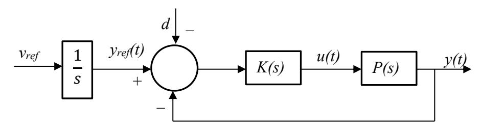
Figure 3. Vehicle's position control system

where d is the distance inter-vehicle. Assumed d = 0, and \(v_{ref} > 0\) the Laplace form of y(t) under PID controller (3) is given by

\[Y(s) = \frac{K_3 \omega_n^2 s^2 + K_1 \omega_n^2 s + K_2 \omega_n^2}{s^3 + (2\zeta \omega_n + K_3 \omega_n^2) s^2 + K_1 \omega_n^2 s + K_2 \omega_n^2} Y_{ref}(s)\](8)

From the transfer function (8), a stable internal system can be determined as \(2\zeta \ge \frac{K_2}{\omega_n K_1} - K_3\) with steady-state error given by \(e_y(t) = sE_y(s) = 0\)

2.2 Intervehicle Distance Control

Assume N vehicles are moving in line and sensors are installed at the vehicle. A group of N vehicles \(\{y_i(t), v_i(t)\}_{i=1}^N\) is the variable to be controlled, while \(\{\zeta_i, \omega_{ni}\}\) are the parameters of i-th vehicle. The structure of a platoon is shown in Figure 4. The first vehicle is the leader and the next vehicles are followers. Vehicle (i+1) follows vehicle i, while the sensor of vehicle i gives the distance information to vehicle (i+1).

Figure 4. Structure of vehicle platoon

In terms of each vehicle, the closed loop transfer function from \(y_{refi}(t)\) to y(t) is given by

\[\frac{y_i(s)}{y_{refi}(s)} = \frac{K_{3i}\omega_{ni}^2 s^2 + K_{1i}\omega_{ni}^2 s + K_{2i}\omega_{ni}^2}{s^3 + (2\zeta_i\omega_{ni} + K_{3i}\omega_{ni}^2)s^2 + K_{1i}\omega_{ni}^2 s + K_{2i}\omega_{ni}^2}\](9)

Data from the sensors are distance information between two vehicles, \(d_i\), given by (10) are often have small error

\[d_i = y_{i-1}(t) - y_i(t) \; ; \; i \ge 2\] (10)

By using the same method used in the transfer function (8), the transfer function of the N-th vehicle (9) will be stable for \(2\zeta_i \geq \frac{K_{2i}}{\omega_{ni}K_{1i}} - K_{3i}\), then \(\lim_{t \to \infty} v(t) = v_{ref}\) and \(\lim_{t \to \infty} y_{i-1}(t) - y_i(t) = d_{ref}\) for all \(i \geq 2\)

The transfer function for the leader / first vehicle from \(v_{ref1}(t)\) to \(v_1(t)\) can be represented by

\[\frac{V_1(s)}{V_{ref_1}(s)} = \frac{K_{31}\omega_{n1}^2 s^2 + K_{11}\omega_{n1}^2 s + K_{21}\omega_{n1}^2}{(1 + K_{31}\omega_{n1}^2)s^2 + (2\zeta_1\omega_{n1}^2 + K_{11}\omega_{n1}^2)s + K_{21}\omega_{n1}^2}\](11)

The position of the leader can be obtained by integrating the leader's velocity. The leader position can then be stated as

\[Y_1(s) = \frac{K_{31}\omega_{n1}^2 s^2 + K_{11}\omega_{n1}^2 s + K_{21}\omega_{n1}^2}{(1 + K_{31}\omega_{n1}^2) s^3 + (2\zeta_1\omega_{n1}^2 + K_{11}\omega_{n1}^2) s^2 + K_{21}\omega_{n1}^2 s}\](12)

As for followers, the second to N-th vehicles, if \(d_{ref} = 0\) output \(y_i(t)\) will approach \(y_{i-1}(t)\), then the transfer function \(y_{i-1}\) to \(y_i\) can be written as

\[\frac{y_i(s)}{y_{i-1}(s)} = \frac{K_{3i}\omega_{ni}^2 s^2 + K_{1i}\omega_{ni}^2 s + K_{2i}\omega_{ni}^2}{s^3 + (2\zeta_i\omega_{ni} + K_{3i}\omega_{ni}^2) s^2 + K_{1i}\omega_{ni}^2 s + K_{2i}\omega_{ni}^2}\](13)

3 Simulation and Results

From the controller design obtained in the previous discussion, the model will be simulated using five vehicles. The first vehicle is the leader, and the four vehicles behind it are followers. In this simulation, it is assumed that the five vehicles are homogeneous with \(\zeta_i=0.82\) and \(\omega_{ni}=0.2\), and the PID parameters obtained above meet the stability criteria. The parameters are selected proportional gain \(K_{1i}=50\), integral gain \(K_{2i}=10\), and derivative gain \(K_{3i}=40\). In the initial conditions, given a 10-meter distance between vehicles, it is desirable at \(t\to\infty\), that the distance becomes 5 meters. The simulation results include position trajectory, vehicle distance, and velocity response.

The position trajectory of the five vehicles, as shown in Figure 5, shows that each vehicle's trajectory has varying distance between vehicles in the beginning. As time increases, the distance between vehicles becomes the same as expected, according to the velocity response at \(t \to \infty\). Figure 6 shows the distance between the five vehicles. When the distance between vehicles is 10 meters, the simulation results show that the distance between the leader and the second vehicle reaches 5 meters without experiencing a significant overshoot. As the distance from the leader gets farther, the greater the overshoot. Take, for example, the distance between vehicle 4 and vehicle 5. At the initial state, the velocity of vehicle 5 was too fast that it became too close to vehicle 4. Over time, the distance between vehicles becomes the same 5 meters according to the set point.

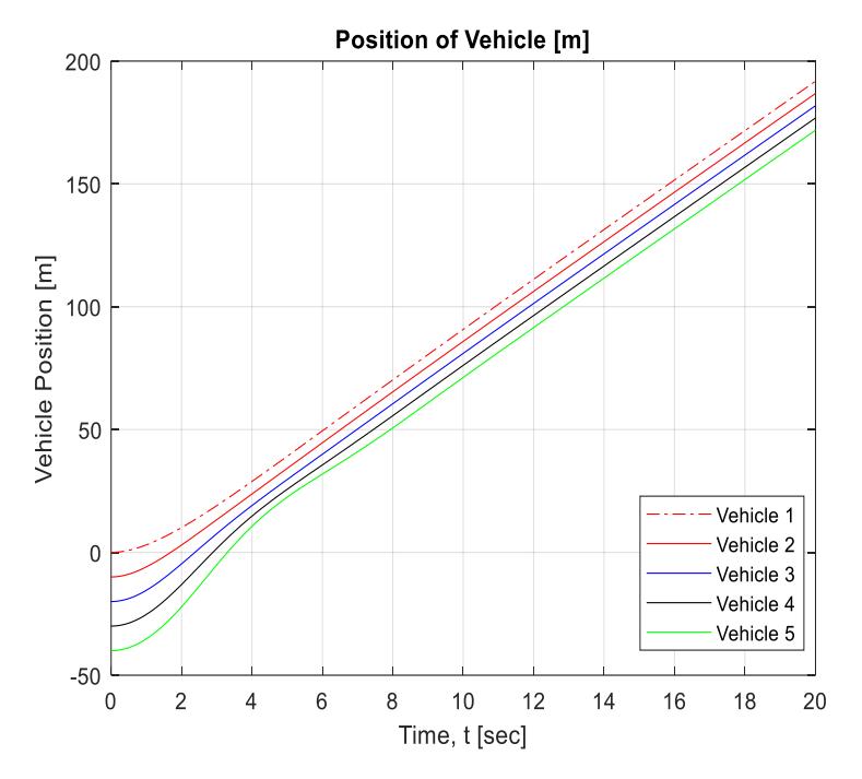
Figure 5. Vehicles trajectory position control

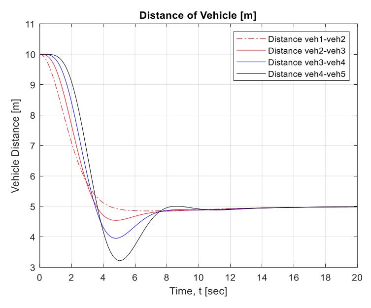
Figure 6. Distance of vehicles

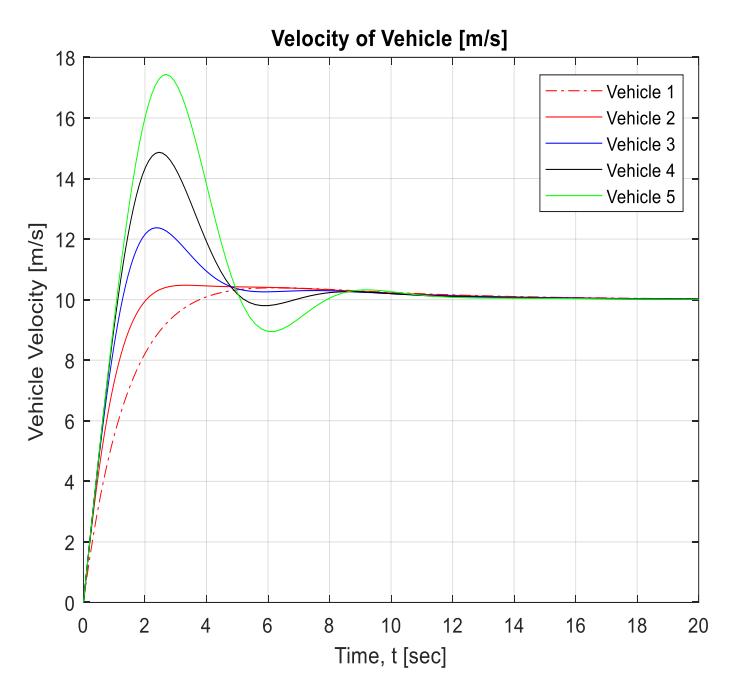
Figure 7. Velocity response of vehicles

Figure 7 shows the velocity response of the five vehicles. It appears that the leader experiences only a small overshoot with a significant rise time. The farther the vehicle's position from the leader, the greater the overshoot, but the faster the vehicle's rise time will be compared to the vehicle in front. The settling time of all vehicles is almost the same, and at t → ∞ all vehicles are the same speed.

4 Conclusion

This paper discusses intervehicle distance control with serial PID control as the controller. A range of parameter values is obtained from the analysis that has been done. This result can be used to make the system stable and the distance between vehicles constant according to the desired set point. However, this modeling and simulation have not included the effects of brake, disturbance, heterogeneous parameters of all vehicles, or uncertainties that occur in actual vehicles. These things will be the next topic of discussion.

5 References

• [1] J. Zhang, T. Feng, F. Yan, S. Qiao, X. Wang, Analysis and Design on Intervehicle Distance Control of Autonomous Vehicle Platoons, ISA Transactions, vol.100, pp. 446-453, May 2020.
• [2] S. Eben and K. Li, Y. Zheng, Y. Wu and J.K. Hedrick, F. Gao, H. Zhang, Dynamical Modeling and Distributed Control of Connected and Automated Vehicles: Challenges and Opportunities, IEEE Intelligent Transportation Systems Magazine, 9(3) pp. 46-58, Oct 2017.
• [3] S.E. Li, K. Li, Y. Zheng, J. Wang, An Overview of Vehicular Platoon Control under the four-componen Framework, IEEE Intelligent Vehicle Symposium (IV), pp. 286-291, June 2015.
• [4] S. Gong, S. Peeta, A. Zhou, Cooperative Adaptive Cruise Control for a Platoon of Connected and Autonomous Vehicles Considering Dynamic Information Flow Technology, Transportation Research Record Journal of the Transportation Research Board, DOI: 10.1177/0361198119847473, March 2019.
• [5] S.E. Li, L.Y. Wang, K. Li, H. Zhang, Platoon Control of Connected Vehicles from a Networked Control Perspective Literature Review, Component Modeling, and Controller Synthesis, IEEE Transactions on Vehicular Technology, DOI 10.1109/TVT.2017.2723881, 2018.
• [6] Y. Zheng, Y. Bian, S. Li and S. E. Li, Cooperative Control of Heterogeneous Connected Vehicles with Directed Acyclic Interactions, IEEE Intelligent Transportation Systems Magazine, doi: 10.1109/MITS.2018.2889654, Jan 2019
• [7] B.D. Schutter, J. Ploeg, L.D. Baskar, G. Naus, H. Nijmeijer, Hierarchical, Intelligent and Atomatic Control, Handbook of Intelligent Vehicles, pp. 81-116, 2012.

• [8] S.E. Li, F.Gao, K. Li, LY. Wang, K. You, D. Cao, Robust Longitudinal Control of Multi-Vehicle Systems – a Distributed H-infinity Method, IEEE Transactions on Intelligent Transportation Systems, vol.19, pp. 2779- 2788, Sep 2018.
• [9] V.D. Khairnar & S,N Pradhan, V2V Communication Survey-(Wireless Technology), Int.J.Computer Technology & Applications, 3 (1), pp. 370-373, Jan-Feb 2012.
• [10]J. Harding, G. Powell, R. Yoon, J. Fikentscher, C.Doyle, D. Sade, M.Lukuc, J. Simons & J Wang, Vehicle-to-Vehicle Communications: Readiness of V2V Technology for Application, (Report No. DOT HS 812 014). Washington, DC: National Highway Traffic Safety Administration, August 2014.
• [11]C. Bergenhem, E. Hedin & D. Skarin, Vehicle-to-vehicle Communication for a Platooning System, Procedia Social and Behavioral Science, 48, pp. 1222-1233, 2012.