
Introduction
The combustion of fossil fuels has led to a substantial increase in carbon dioxide emissions during the current industrial era. Achieving net-zero emissions by 2050 is a formidable task, considering the continuous growth of the economy and population. Global support is essential to harness energy from natural resources, such as solar energy [1]. In the pursuit of carbon neutrality by 2050, renewable energy, particularly solar energy, emerges as a crucial and efficient solution among clean energy sources. It is anticipated to contribute to half of the emission savings by 2030 in the journey toward net-zero emissions [2]. In recent times, photovoltaic array systems have gained recognition and are widely used in electrical applications. Photovoltaic (PV) modules act as the fundamental power conversion units in PV system generators. The output characteristics of PV modules are influenced by solar insulation, cell temperature, and PV module output voltage. PV systems inherently exhibit nonlinear I-V and P-V characteristics that vary with radiation intensity.
System operators face the technical and financial challenges posed by the intermittent nature of PV output, especially with the growing integration of solar energy into the power system. As an uncontrollable generation source, solar energy affects the power system's technical and financial aspects. The stochastic nature of PV systems' output, combined with the likelihood of PV panel failures, transforms the output of PV systems into a stochastic variable. Therefore, the comprehensive development of reliability models for PV systems is crucial in studying solar energy integration and the reliability assessment of power systems. Reliability study methods that simultaneously model solar radiation intensity, PV system equipment, and load demand are expected to address these challenges [3] efficiently.
Reliability analysis of PV systems is vital for system planning, long-term operations, risk assessment facilitation, and limiting income loss [4]. One of the reliability assessment indices for PV is the Loss of Load Probability (LOLP). LOLP can measure the risk of load loss per hour or consider the expected peak load during the dispatch period. Power insufficiency occurs when the system demand exceeds the capability of the operative generation [5], [6]. Using sufficient and high-quality data is crucial to enhance modeling accuracy and reliability assessment [7]. This study utilizes data from the PV system field at the ITB Energy Management Laboratory. Methods such as Markov, Naive Bayes (NB), and Support Vector Machine (SVM) will be employed to assess the reliability of PV systems by identifying possible events that may cause system failures and calculating the probability of the outcomes of these events. The research aims to determine the probability of
power loss due to the PV system's inability to meet load requirements, fulfill the increasing energy needs, and advocate for a better environmental outcome.
Novelty of the Present Study
This study evaluates a microgrid photovoltaic system on a campus building using mathematical analysis and Machine Learning (ML). The reliability of the system is assessed through mathematical analysis, while ML is employed to understand and predict the availability of photovoltaic power based on solar irradiance and consumer demand. This innovative research integrates both methods, which are not commonly practiced in evaluating photovoltaic systems. The ML evaluation results can be implemented in real-time for microgrid management, ensuring accurate and adaptive monitoring based on solar irradiance conditions and electricity consumption. Besides offering practical benefits, this study contributes to the advancement of knowledge in applying mathematical analysis and ML to renewable energy.
Literature Review
The global pursuit of sustainable energy solutions, driven by the imperative of achieving net-zero emissions by 2050, has propelled research into integrating photovoltaic (PV) systems and microgrids. Adefarati et al. [8] laid a crucial foundation by exploring microgrid power systems' reliability and economic dimensions, underscoring the necessity for a comprehensive evaluation framework. Building upon this groundwork, Ayesha et al. in [9] extended the scope by providing insights into the reliability evaluation of energy storage systems, offering a comprehensive review of grid flexibility options. The year 2021 saw Elazab et al. [6] focusing on the reliable planning of isolated Building Integrated Photovoltaic systems, emphasizing the importance of robust planning for standalone systems in achieving sustainability. In 2019, Esan et al. [10] delved into the reliability assessments of an islanded hybrid PV-diesel-battery system, explicitly addressing challenges in rural communities and off-grid applications. The methodological aspects of reliability assessments were enriched by Grandini et al. in [11], who presented an overview of metrics for multi-class classification, contributing theoretical foundations for evaluating classification models.
Moving into 2020, Masih and Verma [12] optimized and evaluated the reliability of hybrid solar wind energy systems, highlighting the significance of combining multiple renewable sources for enhanced reliability. In the subsequent year, Nyamathulla et al. [13] provided an overview of lifetime assessment for multilevel inverters in grid-connected solar photovoltaic applications, shedding light on the longevity and reliability of power electronics in PV systems. Obeidat and Shuttleworth [14] contributed to the reliability prediction of PV inverters, emphasizing the critical components of photovoltaic systems. In 2021, Ostovar et al. [3] presented a reliability assessment of distribution systems integrating photovoltaic and energy storage, addressing the challenges of decentralized energy systems. Concurrently, Paleti [15] contributed to the optimization and reliability evaluation of hybrid power systems, emphasizing the importance of a holistic approach to system design. The year 2020 saw Putri and Adrianti [5] focusing on calculating photovoltaic reliability for assessing the Loss of Load Probability, providing a practical metric for system performance. Raghuwanshi and Arya [16] assessed the reliability of standalone hybrid photovoltaic energy systems, particularly for rural healthcare centers, addressing the unique challenges of remote applications. The year 2023 witnessed Sonawane et al. in [4] performing reliability and criticality analysis of a large-scale solar photovoltaic system, employing fault tree analysis for a comprehensive assessment.
Delving into the theoretical underpinnings of reliability, Syrbe in [17] provided insights into the foundational understanding of the reliability of systems, contributing to the theoretical aspects of system reliability. Urgun and Singh [18] showcased innovative approaches to reliability analysis and proposed a hybrid Monte Carlo simulation and multi-label classification method for composite system reliability evaluation. They further advanced their work in 2020 by incorporating deep learning enhanced by transfer learning for composite system reliability analysis [7]. As the narrative unfolds, Basha et al. [19] introduced machine learning, specifically the Support Vector Machine, in automatic sleep stage classification in 2021, showcasing the adaptability of ML techniques in diverse fields. Finally, Zhang et al. [20] demonstrated the versatility of machine learning techniques in fault detection, applying Naive Bayes for bearing fault diagnosis. These sequential advancements provide a comprehensive overview of the evolving landscape in the reliability evaluation of photovoltaic systems and microgrids, incorporating technological innovations and methodological diversifications over the years.
Experimental Methodology
The research methodology was meticulously chosen to involve the application of mathematical analysis in assessing the failure rate of the system and the probabilistic failure rate of the generator, specifically considering solar irradiance availability. Machine learning techniques were employed to enhance the evaluation of the microgrid's reliability. System analysis critically relies on the evaluation of reliability. This assessment often adopts a probabilistic methodology [9], which can be further classified into analytical and simulation-based approaches. The analytical approach necessitates the use of mathematical models and direct calculations to derive reliability indices. On the other hand, simulation-based methods employ simulations to replicate the random behavior of each system component based on their repair and failure rates.
Table 1. Failure and repair rate of various components [12], [14], [16], [21] [27]
| No | Reliability index | 𝜆 Failure rate ( ) 𝑦𝑒𝑎𝑟𝑠 | Repair time (r) in hours |
|---|---|---|---|
| 1 | PV array | 0,05 | 30 |
| 2 | PV Inverter | 0,0163 | 26,797 |
| 3 | Switch | 0,08 | 24 |
| 4 | Battery | 0,01 | 10 |
| 5 | Inverter | 0,095 | 50 |
| 6 | Main grid | 0,041 | 0,078 |
1 Reliability Evaluation
In this study, the analytical approach employs the Markov model, while the simulation method involves the application of Machine Learning (ML) to estimate the probability of each component's behavior. The evaluation of components encompasses the scrutiny of their failure rates, repair rates, and overall failures, shown in Equations (1), (2), and (3), respectively, taking into consideration the intermittent characteristics of the solar power source [12], [16].
\[P(t) = \lambda \cdot e^{-\lambda t} \tag{1}\]
\[Q(t) = \mu \cdot e^{-\mu t} \tag{2}\]
The reliability of the component is determined as
\[R(t) = \lambda \cdot e^{-\lambda t} \tag{3}\]
Based on the Markov model, the time-dependent availability (AV) and unavailability (UV) are represented as [13].
\[AV(t) = \frac{\mu}{\lambda + \mu} - \frac{\mu}{\lambda + \mu} \cdot e^{-(\lambda + \mu)t}\] (4)
\[UV(t) = \frac{\lambda}{\lambda + \mu} - \frac{\lambda}{\lambda + \mu} \cdot e^{-(\lambda + \mu)t}\] (5)
Considering long-term operation, the steady-state availability (AV) and unavailability (UV) is typically expressed as:
\[AV(t) = \frac{\mu}{\lambda + \mu} \tag{6}\]
\[UV(t) = \frac{\lambda}{\lambda + \mu} \tag{7}\]
Typically, given that µ" λ, the unavailability is expressed as:
\[UV(t) = \frac{\lambda}{\mu} = \lambda \cdot r \frac{hrs}{yr} \tag{8}\]
\[r = \frac{1}{\mu} \tag{9}\]
= 8760 ℎ (10)
2 Reliability indices
The indicators utilized for the reliability of the power supply system in the microgrid include Loss of Load Probability (LOLP), Loss of Load Expectation (LOLE), Expected Energy Not Supplied (EENS), and Energy Index of Reliability (EIR). The performance metrics employed for the reliability assessment in this study are briefly explained as follows [10]. Loss of Load Probability (LOLP)
\[LOLP = \frac{U_{system}}{8760} \tag{11}\]
Loss of Load Expectation (LOLE) is represented as [14]
\[LOLE = 365 \cdot LOLP \tag{12}\]
Expected Energy Not Supplied (EENS) is shown as [16]
\[EENS = L_{average} \cdot U_{system} (\frac{kWh}{years})\] (13)
The Energy Index of Reliability (EIR) is determined by [15]
\[EIR = 1 - EENS \tag{14}\]
3 Markov Model
The Markov model is utilized to evaluate the simulation frequency and duration within uncertain Photovoltaic (PV) systems. This model establishes connections between state probabilities and their associated frequencies and durations. It portrays a system with operational (UP) and failure (Down) states, employing nodes and branches to depict different states and their transition probabilities, as shown in Figure 1. The model's failure rate (λ) represents the likelihood of transitions from operational to failure states, while the repair rate (µ) denotes the reverse transition [21].
Figure 1. Microgrid system reliability network diagram
\[UV_{system} = \lambda_{system} . r_{system}\] (15)
In this context, is indicative of system unavailability, reflecting the degree to which the system is nonoperational. represents the system failure rate, denoting the frequency at which the system experiences failures within a specific time frame. Meanwhile, signifies the average duration of interruption or downtime encountered by the system. Essentially, serves as a metric for gauging how often and for what duration the system undergoes failures or operational disruptions.
This system consists of several main components that work together to ensure a reliable power supply in the microgrid of the campus area. Firstly, there are Photovoltaic (PV) panels, which capture sunlight and convert it into electricity [16]. These panels are essential for the renewable energy generation of the system, providing a sustainable source of electrical power. Along with the PV panels, a switch facilitates the management of electrical flow within the system. This switch allows seamless transitions between various electrical power sources or operational modes, ensuring optimal performance. The PV electricity generated by the panels is converted from direct current (DC) to alternating current (AC) by the PV inverter. This conversion enables compatibility with standard electrical equipment and a broader electrical grid. Additionally, the system includes
battery storage, which stores excess electricity generated by the PV system. This stored energy can be utilized during periods of low sunlight or high demand, enhancing the reliability and resilience of the system.
Furthermore, the system is equipped with a hybrid inverter, which combines the functions of a PV inverter with the battery and main grid. The main grid serves as an essential component, providing additional power supply when needed and enabling the exchange of electricity with a broader electrical grid. This integration allows for efficient management and utilization of the electricity generated by the PV system, with the main grid serving as backup power and electricity stored by the battery within the system. The system comprises a Photovoltaic, switch, PV inverter, battery storage, hybrid inverter, and main grid. This system organizes all subsystems in series and parallel configurations [16]. The reliability network diagram, illustrated in Figure 2, depicts the arrangement of these subsystems.
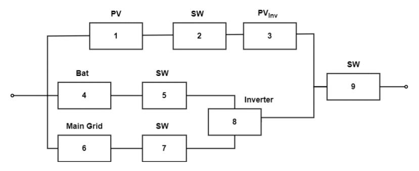
Figure 2. Microgrid system reliability network diagram
The reliability model for a series system consisting of two elements is depicted in Figures 3a, 3b, and 3c. The formula is provided as follows [12]:
\[\lambda_{series} = \sum_{i=1}^{n} \lambda_i \tag{16}\]
E-ISSN: 2460-6340
\[r_{series} = \frac{\sum_{i=1}^{n} \lambda_i \cdot r_i}{\sum_{i=1}^{n} \lambda_i}\] (17)
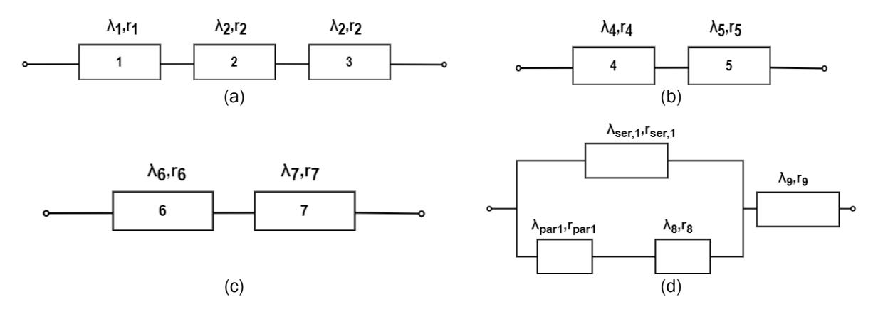
Figure 3. Components system (a) Series (b) Series-parallel
In Figure 3d, we present an illustration of the reliability model for a parallel system consisting of two elements. The formula for evaluating indices in a parallel configuration for battery and main grid is expressed as follows:
\[\lambda_{paralel,1} = \lambda_{ser,2} \lambda_{ser,3} (r_{ser,2} + r_{ser,3})\] (18)
\[r_{par,1} = \frac{(r_{ser2} \cdot r_{ser3})}{(r_{ser2} + r_{ser3})} \tag{19}\]
The configuration in Figure 3b can be expressed mathematically as:
\[\lambda_{paralel,2} = \lambda_{ser} \lambda_{par,1} \lambda_8 (r_{ser} + r_{par,1} + r_8)\] (20)
\[r_{par,2} = \frac{(r_{ser} \cdot r_{par,1} \cdot r_8)}{(r_{ser} + r_{par,1} + r_8)}\](21)
The last obtained failure rate, repair time, and overall system unavailability are as follows, respectively:
\[\lambda_{system} = (\lambda_{par.2} + \lambda_9) \tag{22}\]
\[UV_{system} = (\lambda_{par.2} \cdot r_{par,2} + \lambda_9 r_9)\] (23)
\[r_{par} = \frac{UV_{system}}{\lambda_{system}} \tag{24}\]
Naive Bayes
Machine Learning (ML) is employed for the analysis of power system reliability, specifically in estimating reliability indices like Loss of Load Probability (LOLP). ML is used effectively to predict how a system will behave when random conditions occur. In ML, each sample system status \(C_i < L_i\) reflects whether a loss of load occurs or not.
\[C_i \ge L_i \begin{cases} Success, if \ true \\ Failure, \ else \end{cases}\] (25)
If the Total Number of Failures (TNF) is known using ML, then we can calculate LOLP by dividing it by the Total Number of Samples (TNS), as shown in [18]
\[LOLP = \frac{TNF}{TNS} \tag{26}\]
ML efficiently represents the probabilistic behavior of a microgrid system based on fluctuating solar radiation, providing flexibility in addressing the uncertainty of assessing power system reliability. Reliability is complemented by the probability of failure [17]
\[R = 1 - F \tag{27}\]
Bayes' theorem is applied in the classification problem to utilize Naive Bayes as one of the statistical approaches for inductive inference [20]. If L represents a hypothesis, and N denotes data situated within a specific F class, then P(L|N) is termed the posterior probability, expressing the confidence level in hypothesis L after the provision of data N. The preliminary probability of L for all sample data is denoted as P(L). PP(L|N) is considered notably more informative than P(L). The connection between P(L|N), P(L), and P(N)is elucidated by Bayes's theorem, illustrated as
\[P(L|N) = \frac{P(N|L)P(L)}{P(N)}\] (28)
By the utilization of Bayes's theorem, the Naive Bayes Classifier can be expressed as
\[P(F_i|N) = \frac{P(N|F_i)P(F_i)}{P(N)}\] (29)
The unchanging probability of dataset N for all classes is represented by P(N). \(P(F_i)\) signifies the number of training instances in class Fi/q (q being the number of training data instances). In this scenario, \(P(N|F_i)\). \(P(F_i)\)is a component that can be optimized to achieve an optimal \(P(F_i|N)\), given P(N) and \(P(F_i)\) remain constants. Formulated from these assumptions, \(P(N|F_i)\) is represented as shown
\[P(N|F_i) = \prod_{t=1}^{n} P(n_t|F_i)\] (30)
Here, \(n_t\) signifies the value of the attribute sample N. The probability value \(P(n_t|F_t)\) can be estimated from the training samples.
Support Vector Machine 5
In Support Vector Machines (SVM), the objective is to determine the best possible line (hyperplane) that establishes the widest margin between distinct categories in the dataset. This margin is defined by support vectors, which are the points closest to the line. For Linear SVM, the construction of this line involves weights \((\omega)\) and bias (b), where \(\omega^T X + b = 0\). This line is utilized to classify data points. When discussing the nonlinear version (Nonlinear SVM), a technique known as the kernel trick is employed to handle more intricate patterns in the data. The function f(x) = sign(dis(x)) determines whether a point belongs to one class or another. The distance function dis(x) takes into account support vectors and their impact on the decision. In simpler
terms, SVM strives to establish an optimal boundary between different classes, and this boundary can be either a straight line (Linear SVM) or a more complex curve (Nonlinear SVM), as shown in Figure 4. The decision depends on the nature of the data [19].
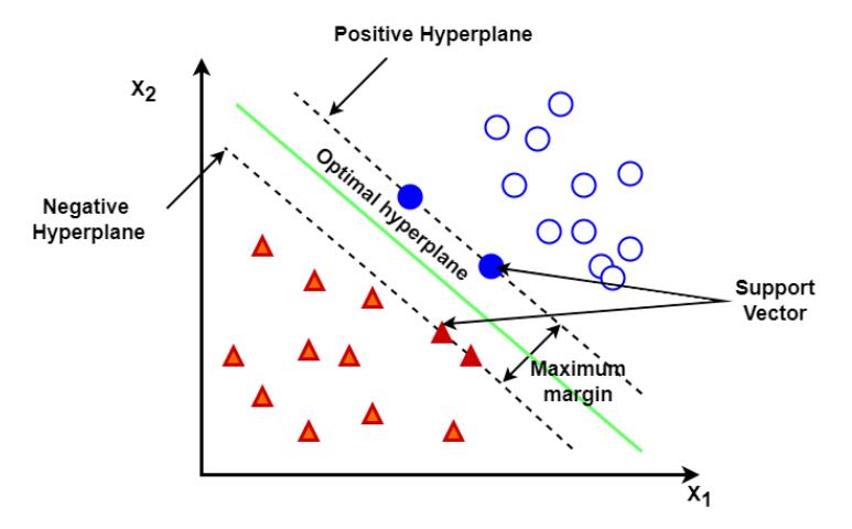
Figure 4. Hyperplane
6 Evaluation Metrics
In this study, evaluation metrics such as Sensitivity, Specificity, Recall, and Accuracy are crucial in assessing the performance of SVM and Naive Bayes models in classifying failure and success states in power generation systems [18], [7], [22]. Sensitivity measures how well the model identifies "failure state" conditions. Its relevance is evident in each False Negative, demanding further analysis by the ML algorithm [7].
\[Sensitivity = \frac{TP}{TP + FN} \tag{31}\]
The Specificity evaluates how accurately the model classifies "success state" conditions. Specificity reflects the precision of classifying normal conditions with a generator probability more significant than the load.
\[Specificity = \frac{TN}{TN + FP} \tag{32}\]
The Recall is essential in identifying all actual system failures, especially when failures have significant consequences [9], [23].
\[Recall = \frac{TP}{TP + FN} \tag{33}\]
The Accuracy is measured by comparing the model's predictions with the actual system states [11], [23].
\[Accuracy = \frac{TP + TN}{TP + TN + FP + FN} \tag{34}\]
Experimental Setup
A microgrid is a power distribution system that caters to the electrical needs of a small, autonomous community, incorporating one or more distributed generators utilizing renewable energy sources. This research focuses on the configuration of the microgrid in the Bandung Institute of Technology, Energy Management Laboratory, as depicted in Figure 5. The microgrid's main components are interconnected with the grid, involving a photovoltaic system, battery energy storage, loads, and a control system [8].
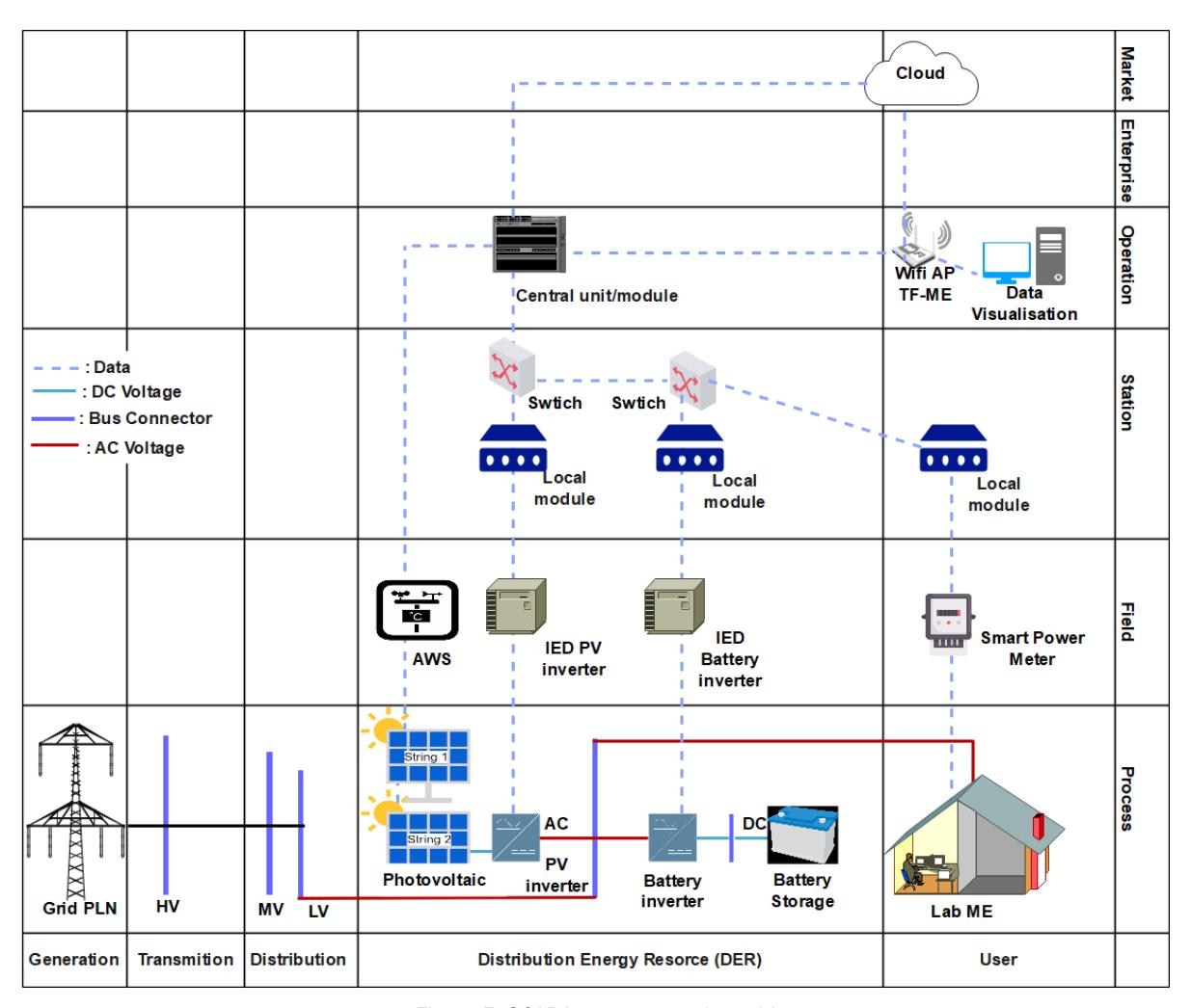
Figure 5. SCADA system on microgrid
The power output measurement system from solar panels (PV) in a microgrid system and the loads shown in Figure 6 within that system, as described in the research by Friansa et al. in [24] and Haq et al. in [25]. The Intelligent Electronic Device (IED) comprises a power monitor, communication interface, and embedded system, serving as a local data concentrator [26].
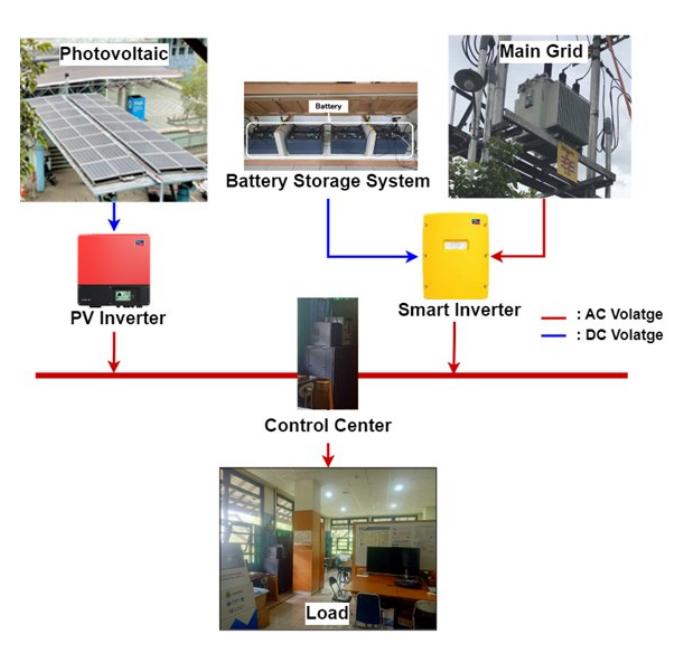
Figure 6. Microgrid power system
The process of modeling microgrid reliability indices begins with collecting raw data containing relevant information for analysis. Subsequently, the data undergoes cleaning and preprocessing stages to address inconsistencies, missing values, and errors. Afterward, the cleaned dataset is categorized into success and failure categories based on predefined criteria. Two classification algorithms, Support Vector Machine (SVM) and Naive Bayes, are then applied to build models based on the categorized dataset. Evaluation is conducted to assess the performance of both models using appropriate evaluation metrics such as Accuracy, Precision, Recall, and F1-score. The process concludes after the evaluation of the models is completed, as depicted in Figure 7.
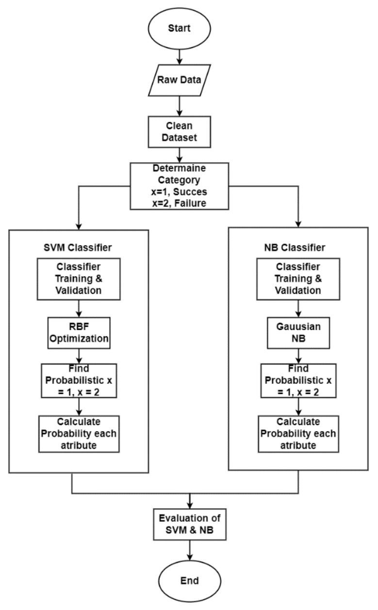
Figure 7. Flowchart ML modelling
Experimental Result
The Photovoltaic System at the Energy Management Laboratory (EML) of Bandung Institute of Technology, Indonesia, is located at a latitude of 6.89, longitude of 107.61, and an altitude of 770 meters. The average solar radiation intensity experienced is 141 Wh/m²/day, as Figure 8a shows monthly solar radiation averages.
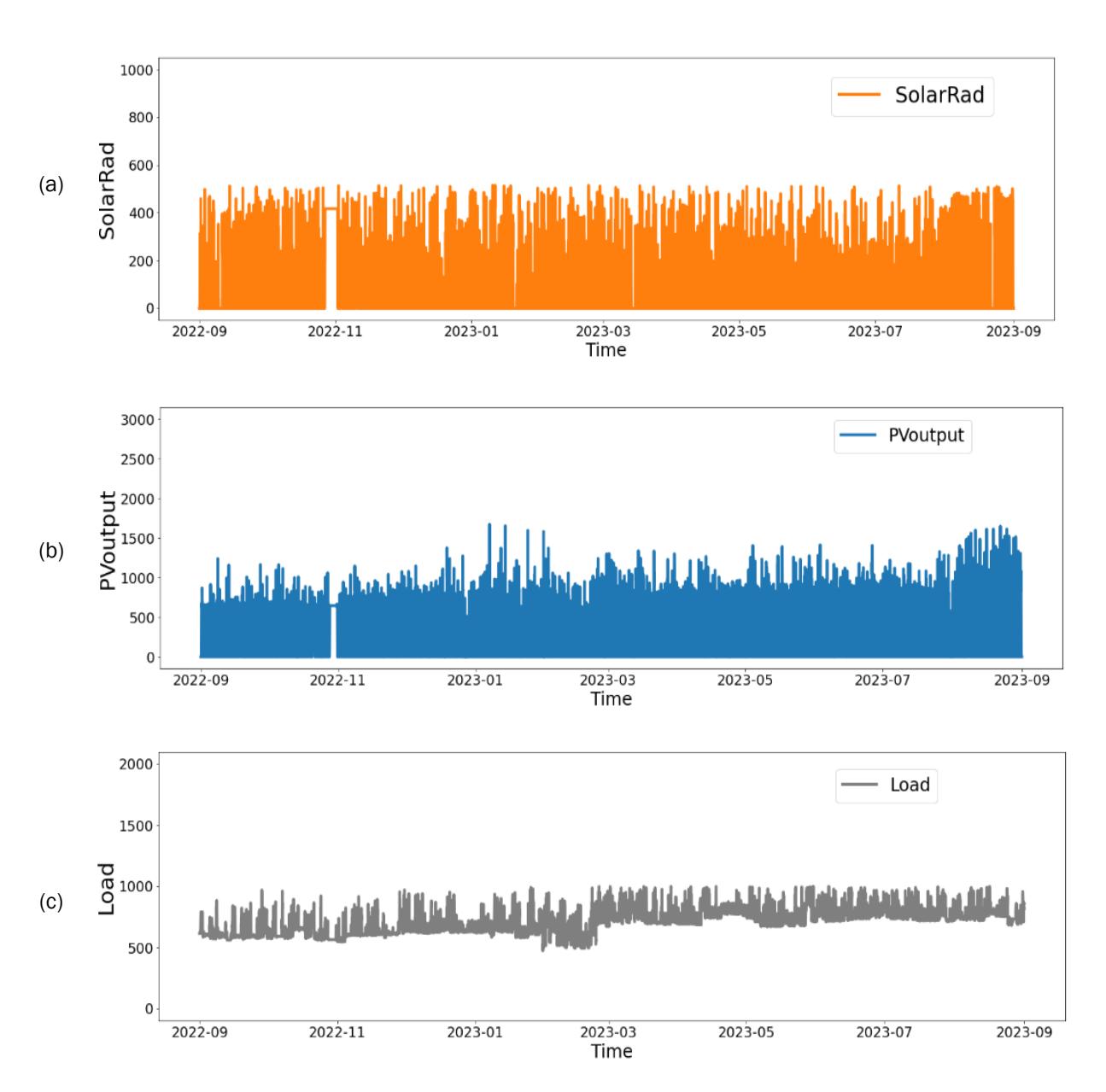
Figure 5. Data system microgrid (a) Irradiance (b) PV output (c) Load
The power demand at EML includes various electrical appliances such as lights, TVs, computers, servers, and other electronic devices. The average hourly power consumption is 710 W, covering AC devices that require an inverter and battery backup. Figure 8c presents a daily overview of the power consumption profile for reliability analysis.
In the isolated operation mode, the average solar radiation fluctuates daily. On January 1, 2024, solar radiation was recorded at 70.13 Wh/m²/hour, resulting in a PV output power of 225 W with a recorded load power of 770 W. A noticeable imbalance exists between the power generated by the PV system and the power demanded by the load. Consequently, surplus power is stored in the battery. If the battery capacity proves insufficient, the system seamlessly transitions to the On-grid mode. The adjustment of operational modes is efficiently managed by the Control Center (CC).
It is crucial to note that PV performance is subject to nonlinear parameters, demonstrating a positive correlation with solar radiation and a negative correlation with temperature. A specific frequency range can be injected into the load within this microgrid system. Deviating from this range is considered a compromise in the reliability of the PV system. To ensure the reliability of the acquired data, we initially conducted data reconciliation and cleaning using the IQR method. The data obtained through this process will be instrumental in evaluating the reliability of the PV system through simulation methods.
Result and Discussion
Evaluating reliability indices requires a comprehensive modeling of all components within the microgrid system. There is both a serial and parallel arrangement within the energy system. Figure 2 illustrates the presence of a switch that initiates operation in on-grid mode when energy is unavailable in isolated mode. Results of the reliability assessment reveal the failure and repair rates of the PV system in the microgrid, documented in Table 2. The reliability index of the serial-parallel system is calculated using the Markov model, as shown in equations (16 to 18), and the output is presented in Table 2. The Reliability Index computation is based on isolated mode conditions.
Table 2. Reliability indices are based on different configurations using the Markov model.
| No | Reliability index | Isolated | On-Grid |
|---|---|---|---|
| 1 | 𝜆𝑠𝑦𝑠𝑡𝑒𝑚/𝑦𝑟𝑠 | 2,805 | 0.575 |
| 2 | 𝑟𝑠𝑦𝑠𝑡𝑒𝑚(ℎ𝑟𝑠) | 15,64 | 12,36 |
| 3 | 𝑈𝑉𝑠𝑦𝑠𝑡𝑒𝑚(ℎ𝑟𝑠/𝑦𝑟𝑠) | 43,592 | 7,107 |
| 4 | 𝑀𝑈𝑇 | 0,3565 | 1,7391 |
| 5 | 𝐿𝑂𝐿𝑃 | 0,0050 | 0,0008 |
| 6 | 𝑑𝑦𝑠 𝐿𝑂𝐿𝐸( ) 𝑦𝑟𝑠 | 1,8285 | 0,2961 |
| 7 | 𝑘𝑊ℎ 𝐸𝐸𝑁𝑆( ) 𝑦𝑒𝑎𝑟 | 31,124 | 5,069 |
| 8 | 𝐸𝐼𝑅 | 0.956 | 0,9928 |
In isolated mode, the energy system exhibits a failure frequency of 2.805/year, an outage duration of 43.85 hours/year, and an unavailability of 15.64 hours. Conversely, during on-grid operating mode, the failure frequency is 0.575/year, with an outage duration of 7.107 hours/year and an unavailability of 12.36 hours. The LOLP for the energy system is determined to be 0.0050 in isolated mode and 0.0008 in on-grid mode. Additionally, the Energy Not Served (EENS) is calculated at 31.124 kWh/year in isolated mode and 5.069 kWh/year in on-grid mode. These indicate that the on-grid operating mode is more reliable than the isolated mode. The evidence is the significant decrease in failure frequency, outage duration, and system unavailability time in the on-grid mode. Furthermore, the lower LOLP and smaller EENS in the on-grid mode also suggest that the system is more efficient in meeting energy demands and reducing unmet energy when operating in the ongrid mode. Therefore, the on-grid mode may be a preferred option for improving the reliability and efficiency of the energy system.
Table 3. Index evaluation-based solar radiation data
| Index Evaluation | Naive Bayes | Support Vector Machine |
|---|---|---|
| Success States | 2833 | 2413 |
| Failure States | 5927 | 6347 |
| LOLP | 0.6765 | 0.7245 |
| Sensitivity | 0.9979 | 0.9987 |
| Specificity | 0.9978 | 0.9978 |
| Recall | 0.9978 | 0.9978 |
| Accuracy | 0.9566 | 0.9988 |
Table 3 presents an analysis of the reliability of the hybrid PV/Battery energy system utilizing the Machine Learning (ML) method, which is based on LOLP indices and failure rates. The application of ML enables realtime assessments of system reliability. Although the system still exhibits lower reliability due to load consumption surpassing the average available PV power, the ML method proves valuable in providing reliable projections. The assessment results indicate that, annually, the LOLP index values using the ML method are 0.6765 and 0.7245, respectively.
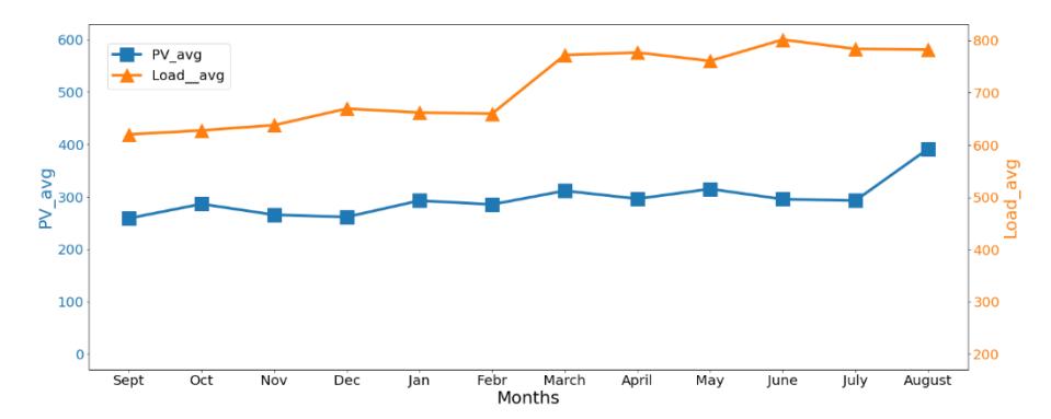
Figure 6. Monthly average PV and Load
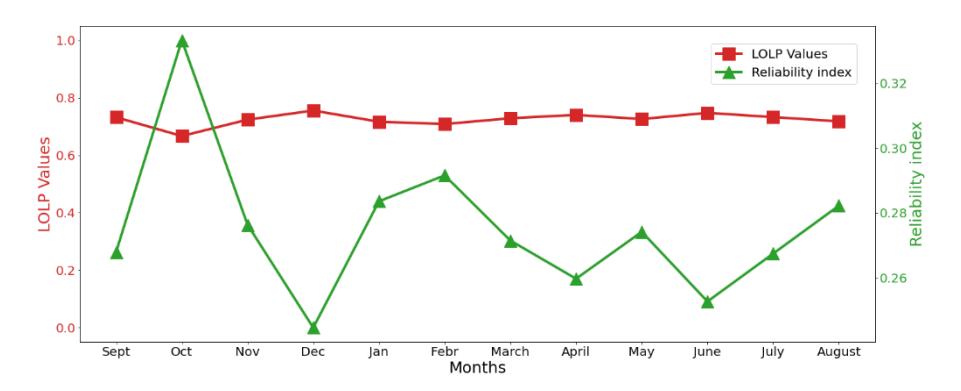
Figure 7. Monthly LOLP and Reliability index
In Figures 9 and 10, an examination of PV power availability is conducted concerning monthly average load requirements and reliability indices. The LOLP is introduced, and the assessment reveals that the reliability index reached optimal levels in October, characterized by low LOLP rates. Nevertheless, during periods outside of October, the system exhibits an average reliability index marked by elevated LOLP rates, as the values do not approach zero. A higher LOLP value, when compared to zero, corresponds to diminished system reliability.
This research presents a more holistic approach to evaluating the reliability of PV systems in microgrids compared to the studies conducted by Widjayanto [21] and Putri [5]. Widjayanto focused on assessing nanogrid reliability using a Markov model, while Putri calculated PV reliability using LOLP calculation and solar irradiance probability methods. However, neither study utilized machine learning (ML) methods to evaluate LOLP in real-time, as this research did. By leveraging ML, this study provides a more dynamic and accurate assessment of system reliability, enabling early detection of potential failures. Additionally, this research presents an analysis of PV power availability to monthly average load requirements and reliability indices, providing a deeper understanding of system performance dynamics.
Conclusions
This research highlights the importance of evaluating the reliability of microgrid systems to ensure a stable electricity supply. The analysis reveals that in isolated operation mode, the system frequently experiences failures, with a frequency of 2.805 per year and a downtime duration of 43.85 hours per year. However, when operating in on-grid mode, both the frequency of failures and downtime duration significantly decrease to 0.575 per year and 7.107 hours per year, respectively. The analysis results using Markov, Naive Bayes, and SVM models confirm that the microgrid system exhibits significant unreliability, especially under conditions of solar radiation availability and PV output not meeting load demand, with a LOLP reaching 0.7245. Nevertheless, in on-grid operation mode, the system components demonstrate high reliability, as evidenced by a very low LOLP of 0.0008. The methodology employed in this manuscript can be implemented in real-time power generation systems to minimize operational costs and energy consumption while enhancing the reliability of the power generation system.