
Abstrak
Industri batik menghasilkan limbah cair dengan pH tinggi akibat penggunaan natrium hidroksida dalam proses pewarnaan, sering melampaui baku mutu pH 6–9. Metode pengenceran tradisional terbukti tidak efisien secara ekonomis, sehingga diperlukan strategi kontrol yang lebih adaptif. Penelitian ini merancang dan mensimulasikan sistem kontrol adaptif nonlinier berbasis Model Reference Adaptive Control (MRAC) untuk netralisasi pH menggunakan asam asetat. Model matematis Continuous Stirred Tank Reactor (CSTR) dikembangkan dari neraca massa, kesetimbangan asam-basa, dan prinsip elektroneutralitas, kemudian disimulasikan menggunakan fungsi Ordinary Differential Equation (ODE) di MATLAB. Kinerja MRAC dibandingkan dengan pengendali PI konvensional pada berbagai kondisi pH awal limbah. Hasil simulasi menunjukkan bahwa MRAC mencapai konvergensi lebih cepat, mencapai pH 7 dalam 2488,68 detik dari pH awal 9, dibandingkan pengendali PI (3080,96 detik) atau sistem tanpa kontrol (10225 detik). Dengan settling time 2377 detik versus 2566,4 detik untuk PI, MRAC mengurangi konsumsi penetral sebesar 0,61% (9,5380 L versus 9,5969 L) sambil mempertahankan kriteria keamanan di atas batas bawah pH 6,80. Analisis stabilitas Lyapunov mengonfirmasi kestabilan asimtotik pengendali adaptif. Penelitian ini menunjukkan bahwa MRAC menawarkan kinerja superior untuk pengendalian pH limbah batik sambil mengurangi ketergantungan pada metode pengenceran yang tidak ekonomis.
Kata Kunci: netralisasi pH, pengolahan limbah, kontrol adaptif, MRAC, kontrol proses kimia.
Paper received October 4th, 2025 – Paper revised January 20th, 2026 – Paper accepted January 26th, 2026
This paper is open access with CC BY-SA license.
1 Introduction
Official recognition from the international organization UNESCO of batik correlates positively with increased market demand and public interest [1]. As the batik industry grows, wastewater volume increases and degrades environmental quality. Batik wastewater generally has characteristics of turbid color, foaming, high pH, high Biological Oxygen Demand (BOD) and Chemical Oxygen Demand (COD) concentrations, as well as oil and grease content. This is caused by the use of chemicals and dyes in the batik production process [2]. Extreme pH values mainly originate from the dyeing and dipping stages where some processes add strong bases and others add acids, so the effluent can be acidic or basic and carry synthetic dye residues. Therefore, equalization tanks and neutralization units are needed so that the final pH returns to the wastewater quality standard range. The pH quality standard for wastewater based on the Regulation of the Minister of Environment and Forestry of the Republic of Indonesia Number P.16/MENLHK/SETJEN/KUM.1/4/2019 ranges from 6–9 [3].
This research aims to design and simulate a nonlinear adaptive control system for the pH neutralization process in batik industry wastewater treatment plant (WWTP). Batik wastewater tends to be strongly basic due to the use of sodium hydroxide in dyeing, scouring, and washing stages, with high variability in flow rate and concentration [4]. Neutralization dynamics in stirred tank reactors are nonlinear due to acid-base equilibrium and buffer effects, making standard PI controllers sensitive to load changes. The control target refers to the pH quality standard of 6–9. Before presenting simulation results and controller comparisons, initial surveys and characterization were conducted to establish operating ranges, process parameters, and performance evaluation reference points.
Surveys and wastewater sampling have been conducted at Komar Batik industry. The batik wastewater samples were also tested for wastewater characteristics at the Water Quality Laboratory, Faculty of Civil and Environmental Engineering, Bandung Institute of Technology. The testing method refers to the Standard Method for The Examination of Water and Wastewater 23rd Edition 2017 (APHA) and Indonesian National Standard 2004 (SNI). The test results showed that the sample pH was 7.07, meaning the wastewater pH met the industrial wastewater quality standards. Therefore, a second survey was conducted with fresh wastewater from the final batik production process. The second survey was conducted at nine batik industries in the Trusmi area, Cirebon, and only three batik wastewater samples were obtained because the pandemic situation at that time caused many batik industries to stop production. Laboratory test results showed that two of the three wastewater samples obtained from hand-drawn batik industries had pH values of 9.32 and 10.1. This means the wastewater pH did not meet the quality standards for environmental discharge. Meanwhile, one other sample obtained from stamp batik industry had a pH of 7.89, meaning the wastewater pH met the requirements for discharge. This is addressed by batik producers by continuously flowing water during the final production process so that the wastewater content consists of 70% water and 30% batik wastewater [5]. In other words, water pumps are kept running all day; if this continues, it will be economically burdensome due to increasingly expensive electricity costs. Producers are aware of this situation—from a production perspective, they get little profit, while distributors get more profit by selling batik at higher prices compared to what producers sell.
Based on the survey and laboratory testing results, it can be concluded that some batik wastewater, especially from hand-drawn batik industries, has pH levels exceeding quality standards and therefore requires treatment before environmental discharge. This condition drives the need for designing efficient pH control systems to reduce dependence on uneconomical dilution methods using clean water. For this purpose, pH neutralization process simulation was conducted as the initial stage of control system development. This simulation was built using Ordinary Differential Equation (ODE) functions in Matlab with a neutralization process volume capacity adjusted to the plant tank size of 87.75 liters, so it can represent real field conditions.
2 Methodology
This section presents the research stages in sufficient detail to allow reproduction. The study was conducted on batik wastewater containing sodium hydroxide (NaOH) as the alkaline stream and acetic acid (CH₃COOH) as the neutralizing agent. The neutralization process was modeled using a continuous stirred-tank reactor (CSTR) framework implemented in Matlab with numerical differential equation solvers. The methodology includes reaction modeling and process flow analysis, the development of a simulation framework to compare control strategies, the design and simulation of conventional PI and adaptive MRAC controllers, and stability analysis based on Lyapunov theory to ensure the reliability of the control system's performance.
2.1 pH Neutralization Process
Neutralization is a reaction between acid and base solutions to achieve target pH [6], [7], [8], [9]. Batik wastewater is strongly basic due to the use of caustic soda (NaOH) in the dyeing process. In water, NaOH dissociates completely producing OH⁻ ions. To neutralize it, a weak acid is chosen, namely acetic acid
(CH₃COOH), because it is easily obtained and relatively safe for the environment compared to HCl and H2SO4 [10]. The process flow diagram (PFD) for pH neutralization is shown in Figure 1.
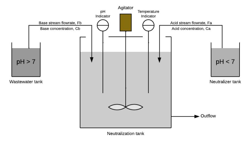
Figure 1. Process flow diagram of pH neutralization [10], [11].
2.2 Simulation Flow of pH Neutralization Process
Figure 2 shows the flowchart of simulation stages conducted to analyze and compare the performance of two control methods in the pH neutralization process, namely conventional PI controller and adaptive controller. The process begins with initialization of parameters and simulation scenarios, then builds a mathematical model of the pH neutralization process used as reference. After analyzing the system in open-loop conditions, both controller methods are evaluated separately. For the PI controller, parameter tuning is performed, while for the adaptive controller, identification and adaptive parameter adjustment stages are conducted. Each controller is then simulated, its performance metrics measured, and results compared to determine control effectiveness in the system.
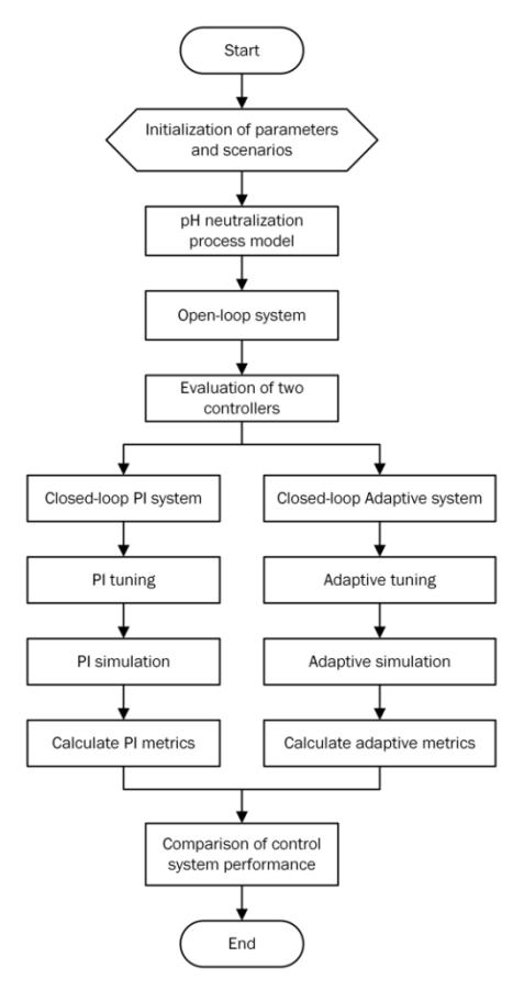
Figure 2. Simulation flowchart of pH neutralization with two controller strategies.
2.3 Design of the pH Neutralization Process Control System
The design of an effective control system for pH neutralization in batik wastewater treatment must consider the strong alkalinity of the wastewater (pH > 9) resulting from sodium hydroxide used in the dyeing process, as well as the nonlinear acid-base equilibrium dynamics in a continuous stirred-tank reactor (CSTR). To address these challenges, this study develops a comprehensive control framework that begins with mathematical modeling of the neutralization process dynamics, followed by the design and simulation of control strategies, and concludes with stability analysis. Emphasis is placed on comparing the performance of a conventional PI
controller with a Model Reference Adaptive Control (MRAC) scheme, where the adaptive mechanism enables automatic parameter adjustment to enhance robustness and reliability of pH regulation in nonlinear and timevarying systems.
2.3.1 Mathematical Derivation of the pH Neutralization Process Dynamic Model
The dynamics of pH neutralization process was first modeled by McAvoy et al. in 1972 [12]. This model is based on a Continuous Stirred-Tank Reactor (CSTR). Its differential equation is derived from mass balance, acid-base dissociation equilibrium, and electroneutrality condition. This formulation has been widely adopted in subsequent research, including [7], [10], [11], [13]. Therefore, this research also adopts the same pH neutralization process dynamic model and focuses on simulation. The difference lies in the control strategy used, which compares PI controller with Model Reference Adaptive Control (MRAC).
In this research, the wastewater studied contains strong base sodium hydroxide (NaOH) with pH > 9, while the neutralizer is weak acid \(CH_3COOH\). The decomposition reactions of each solution in water are shown by equations (1) and (2).
\[NaOH_{(aq)} + H_2O_{(aq)} \rightarrow Na_{(aq)}^+ + OH_{(aq)}^-\] (1)
E-ISSN: 2460-6340
\[CH_3COOH_{(aq)} + H_2O_{(aq)} \rightarrow CH_3COO_{(aq)}^- + H_3O_{(aq)}^+\] (2)
From the reaction in equation (2), the acid dissociation constant \(k_a\) for \(CH_3COOH\) solution can be calculated through the following acetic acid equilibrium.
\[k_a = \frac{[CH_3COO^-][H^+]}{[CH_3COOH]} = 1,75 \times 10^{-5}\] (3)
The neutralization reaction between the two solutions will produce salt solution and water.
\[NaOH_{(aq)} + CH_3COOH_{(aq)} \rightarrow CH_3COONa_{(aq)} + H_2O_{(l)}\] (4)
\[H_2O_{(1)} \to H_{(aq)}^+ + OH_{(aq)}^-\] (5)
\[k_{w} = [H^{+}][OH^{-}] = 1 \times 10^{-14}\] (6)
The dynamic model used in the pH neutralization process consists of two differentials representing acid and base dissociation processes. This model is influenced by input flows: acid neutralizer inlet flow rate \(F_a\) (L/min), waste inlet flow rate \(F_b\) (L/min), acid concentration \(C_a\) (mol/L), waste concentration \(C_b\) (mol/L), tank volume \(V_t\) (L), parameter \(x_1\) as acid dissociation, parameter \(x_2\) as wastewater dissociation. Equation (7) represents acetate balance, while equation (8) represents sodium balance [10], [14], [15].
\[\frac{\mathrm{dx_1}}{\mathrm{dt}} = \frac{\mathrm{F_aC_a}}{\mathrm{V_t}} - \frac{\mathrm{F_a + F_b}}{\mathrm{V_t}} \mathrm{x_1} \tag{7}\]
\[\frac{dx_2}{dt} = \frac{F_b C_b}{V_t} - \frac{F_a + F_b}{V_t} x_2 \tag{8}\]
In this research, parameter \(x_1\) is acid dissociation influenced by \(CH_3COOH\) and \(CH_3COO^-\), while parameter \(x_2\) is base dissociation or wastewater dissociation influenced by \(Na^+\).
\(x_1 = [CH_3COOH] + [CH_3COO^-]\) (9)
\[x_2 = [Na^+] \tag{10}\]
E-ISSN: 2460-6340
In CSTR, acid and base solutions mix and react to form salt and water. The system always satisfies electroneutrality condition, where total positive charge equals total negative charge at all times. The electroneutrality condition for NaOH and \(CH_3COOH\) mixture is formulated in equation (11).
\[[Na^+] + [H^+] = [CH_3COO^-] + [OH^-]\] (11)
Then if equations (2), (3), (6), and (10) are substituted into equation (11), it will produce a cubic equation as in equation (12).
\[[H^{+}]^{3} + a_{1}[H^{+}]^{2} + a_{2}[H^{+}] + a_{3} = 0\] (12)
\[a_1 = k_a + x_2 (13)\]
\[a_2 = x_2 k_a - k_w - k_a x_1 = k_a (x_2 - x_1) - k_w\] (14)
\[a_3 = -k_a k_w \tag{15}\]
At the end of the pH neutralization process between wastewater and neutralizer can be calculated using equation (16).
\[pH = -\log_{10}[H^{+}] \tag{16}\]
2.3.2 Simulation Design for the pH Neutralization Process Control System
Adaptive is a control system that can automatically adjust parameters to compensate for changes in characteristics of the controlled process. Adaptive controller is needed because most chemical processes are nonlinear and non-stationary (their characteristics change with time), so adaptation procedures are required. Several criteria that can be used, including the one-quarter decay ratio, Integral Square Error (ISE), and gain/phase margin [16].
This research uses MRAC (Model Reference Adaptive Control) structure, where system output follows the performance of its reference model output. The MRAC block diagram is shown in Figure 3.
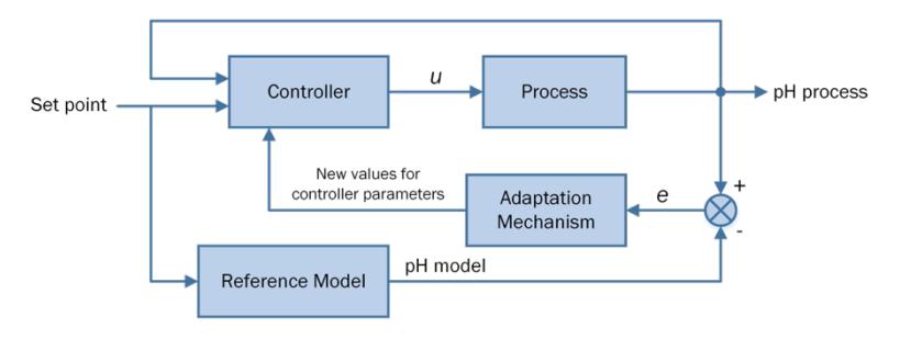
Figure 3. MRAC block diagram
From electroneutrality, we obtain
\[x_0 = [CH_3COOH] + [CH_3COO^-] - [Na^+] = x_1 - x_2\] (17)
By combining equations (7)–(9) and equation (17) [17] then
\[\dot{x}_{p} = \frac{1}{V_{+}} (F_{a}C_{a} - F_{b}C_{b} - (F_{a} + F_{b})x_{p})\] (18)
ps://doi.org/10.5614/joki.2026.18.1.4 E-ISSN: 2460-6340
\(x_p\) can be calculated from weak acid strong base pH process [18] as follows
\[x_{p} = x_{2} - \frac{k_{a}x_{1}}{k_{a} + [H^{+}]} + [H^{+}] - \frac{k_{w}}{[H^{+}]} = 0\] (19)
The reference model equation is stated in equation (20)
\[\frac{dx_{1m}}{dt} = \frac{F_a C_a}{V_t} - \frac{F_a + F_b}{V_t} x_{1m} \frac{dx_{2m}}{dt} = \frac{F_b C_b}{V_t} - \frac{F_a + F_b}{V_t} x_{2m}\] (20)
and model pH,
\[pH_{m} = 14 - pOH \tag{21}\]
Then rewriting equations (18) and (20) gives
\[\dot{x}_{p} = \frac{1}{V_{t}} \left( u \left( C_{a} - x_{p} \right) - F_{b} \left( C_{b} - x_{p} \right) \right) \tag{22}\]
\[\dot{x}_{m} = \frac{1}{V_{t}} (F_{a}C_{a} - F_{b}C_{b} - (F_{a} + F_{b})x_{m})\] (23)
Defining error,
\[e = x_p - x_m \tag{24}\]
Then the controller is expressed as
\[u = \theta_a(\alpha_p - \alpha_m) + \theta_b(pH_p - r)\] (25)
where r is reference input, and adaptation mechanism is stated in equations (26) and (27)
\[\theta_{a} = \frac{\gamma_{1}e(\theta_{b} - pH_{p})}{V_{+}}, \qquad \gamma_{1} > 0\] (26)
\[\theta_{b} = \frac{\gamma_{2}e}{V_{t}}, \qquad \gamma_{2} > 0 \tag{27}\]
2.3.3 Proof of Stability
From equations (22)-(25), we obtain
\[\dot{\mathbf{e}} = -\frac{\mathbf{e}}{V_{\star}} \left( \theta_{a} (\alpha_{p} - \alpha_{m}) + \theta_{b} (pH_{p} - r) - F_{b} \right) \tag{28}\]
To guarantee controller stability, a Lyapunov Function Candidate is chosen with the form of equation(29) which is standard used for stability analysis because its value is always positive for \(e \neq 0\) and V = 0 when e = 0.
\[V = \frac{1}{2}e^2 \tag{29}\]
The stability condition is boundedness, for the system to be stable (especially globally asymptotically stable) the condition \(\dot{V} < 0\) is required for all \(e \neq 0\).
Vol 18 (1), 2026
\(\dot{V} = e\dot{e}\) (30)
E-ISSN: 2460-6340
\[\dot{V} = -\frac{e^2}{V_t} \left( \theta_a \left( \alpha_p - \alpha_m \right) + \theta_b \left( p H_p - r \right) - F_b \right) \tag{31}\]
Based on equation (31), the derivative of Lyapunov function \(\dot{V}\) will always be negative can be achieved if \(V_t > 0\) and \(\theta_a(\alpha_p - \alpha_m) + \theta_b(pH_p - r) - F_b > 0\) for all time, thus satisfying negative-definite property. With controller parameter selection that meets the above conditions, this condition guarantees that Lyapunov function V will decrease monotonically until reaching zero, meaning error e will approach zero over time, so the designed controller can be asymptotically stable according to Lyapunov stability criteria and the system has bounded-input bounded-state (BIBS) property.
2.3.4 Performance Metrics
This subsection defines the quantitative metrics used to evaluate closed-loop performance in terms of tracking accuracy, convergence speed, operational cost, and safety. These indices are computed from the simulated pH response and the manipulated neutralizer flow rate over the simulation horizon \(t \in [0,T]\). In particular, the metrics include integral tracking-error measures (IAE and ISE), settling time for assessing convergence, a lower-bound constraint indicator based on the minimum pH, the total neutralizer volume to represent chemical usage, and a composite cost function that combines safety and economy. These definitions are subsequently used to produce the performance summary in Table 3 and to support the discussion of tradeoffs between the PI and MRAC controllers.
a. Tracking error and integral error indices
Tracking quality is assessed using integral error indices computed from the tracking error in equation (32)
\[e(t) = pH(t) - sp (32)\]
The integral of absolute error (IAE) and the integral of squared error (ISE) are defined in equation (33) and (34).
\[IAE = \int_{0}^{T} |e(t)| dt\] (33)
\[ISE = \int_{0}^{T} e^{2}(t) dt\] (34)
b. Settling time
Response speed is evaluated using the settling time, defined as the earliest time after which the output remains within a ±2% band around the final value.
c. Safety constraint indicators
A lower pH bound is set as LimitLow = \(sp - \delta\), and safety is assessed using the minimum pH in equation (35).
\[pH_{min} = \min_{t \in [0,T]} pH(t)\] (35)
d. Total neutralizer usage
From an operational perspective, chemical usage is quantified by the total injected neutralizer volume as defined in equation (36).
\[V_{N} = \int_{0}^{T} \max(F_{a}(t), 0) dt\] (36)
where \(F_a(t)\) denotes the neutralizer flow rate, and \(max(F_a(t),0)\) ensures that only nonnegative (physically admissible) injection is accumulated.
normalized neutralizer usage V<sub>N</sub>.
e. Composite tradeoff cost function The tradeoff between safety and chemical economy is summarized by a composite cost J, defined as a weighted sum of (i) a normalized penalty for pH excursions below LimitLow (over-acidification) and (ii) the
\[J = W_{0S}J_{0S,n} + W_{\mu}J_{\mu,n} \tag{37}\]
E-ISSN: 2460-6340 with
\[J_{\text{os}} = \int_{0}^{T} [max(0, LimitLow) - pH(t)]^{2} dt, \qquad J_{\text{os},n} = \frac{J_{\text{os}}}{\delta^{2}T}\](38)
\[J_u = \int_0^T \max(F_a(t), 0) dt, \qquad J_{u,n} = \frac{J_u}{F_{a,nom}T}\] (39)
and \(LimitLow = sp - \delta\).
3 Results and Discussion
pH control is performed based on neutralization process influenced by wastewater flow and neutralizer flow entering the neutralization tank. pH neutralization is simulated using Ordinary Differential Equation (ODE) function programmed based on dynamic equations for pH in Continuous Stirred Tank Reactor (CSTR) in Section 2.3.1 derived by McAvoy et al. [12]. Control variables in the pH neutralization process are neutralizer flow rate (\(F_a\)) and neutralizer concentration (\(F_a\)). pH control aims to obtain wastewater results that comply with standards from the Ministry of Environment, namely 6–9 pH [19]. In pH neutralization process simulation, wastewater flow (\(F_b\)) is considered constant and wastewater concentration (\(F_b\)) adjusts to wastewater pH.
3.1 Open Loop Simulation
In this open loop pH neutralization process simulation, weak acid (\(CH_3COOH\)) as neutralizer is mixed with wastewater containing strong base (NaOH). This means only part of the weak acid dissociates into ions in solution, while strong base completely dissociates into ions in solution. Therefore, when neutralizing, only part of the weak acid dissociates to neutralize the solution. Thus, the amount of base neutralized depends on the amount of \(H^+\) released by the weak acid.
Open loop simulation aims to find \(F_a\) and \(C_a\) parameters that will be applied in plant WWTP implementation, while \(F_b\) parameter is considered constant and \(C_b\) adjusts to wastewater pH. Figure 4 shows open loop simulation output of pH neutralization process, with wastewater pH assumed to be 8, 9, and 9.5. Figure 4(a) is simulated with pH 8 parameters, neutralizer flow rate \(F_a = 0.02\) L/min, wastewater flow rate \(F_b = 1\) L/min, and neutralizer concentration \(C_a = 0.0001\) M. Simulation results show that pH can drop towards setpoint pH 7. Then at pH 9 (Figure 4(b)), using the same \(F_a\), \(F_b\), and \(C_a\) parameters as in Figure 4(a), pH from 9 cannot drop towards pH 7. Based on equation (16), pH is determined by logarithmic equation. Therefore, when calculating from pH 7 to 8 to 9, pH 7 has the lowest concentration (\(C_a\)), so at pH 8 the concentration increases 10 times, and at pH 9 the concentration increases 100 times. In other words, from pH 8 to pH 9, concentration increases 10 times. Therefore, the previous acid concentration (0.0001 M) sufficient to reduce from pH 8 to 7 because the concentration increases 100 times.
There are two options to reduce pH from 9 to 7, namely (i) increasing acid flow, and (ii) increasing acid concentration. Next, simulation is performed from pH 9 to 7 with concentration increased to \(C_a = 0.001 \, \text{M}\), \(F_a\) and \(F_b\) parameters still same as in Figure 4(a), pH from 9 can drop but has not reached desired pH as shown by Figure 4(c). If flow rate \(F_a\) is increased 10 times to \(F_a = 0.2 \, \text{L/min}\), then the effect is that pH will drop too far indicating that given \(F_a\) is excessive because it's too large, and from tank construction side it will cause solution in process tank to overflow. Therefore, \(F_a\) needs to be reduced, but must be larger than \(F_a = 0.02 \, \text{L/min}\), so \(F_a = 0.03164 \, \text{L/min}\) is chosen producing pH graph as in Figure 4(d). The same step is applied to neutralize from pH 10 to 7, if want to design appropriate neutralization effect, then acid concentration must be more concentrated, namely \(C_a = 0.01 \, \text{M}\).
Figure 4(e) is simulated with wastewater pH parameters assumed 9.5 and neutralizer flow rate variation between \(F_a=0.1\) L/min to \(F_a=0.1940\) L/min, wastewater flow rate \(F_b=1\) L/min, and neutralizer concentration \(C_a=0.001\) M. Simulation results show that the larger the neutralizer flow rate, the faster the wastewater pH reduction. However, flow rate 0.1940 L/min is the maximum flow rate limit to reduce pH 9.5 to
Jurnal Otomasi Kontrol dan Instrumentasi Vol 18 (1), 2026 ISSN: 2085-2517 https://doi.org/10.5614/joki.2026.18.1.4 E-ISSN: 2460-6340 7, if Fa value exceeds that number then pH will drop far and not in steady state condition. With Fa = 0.1940 L/min, pH can approach setpoint and reach steady state at pH 7.02 in 7549 seconds.
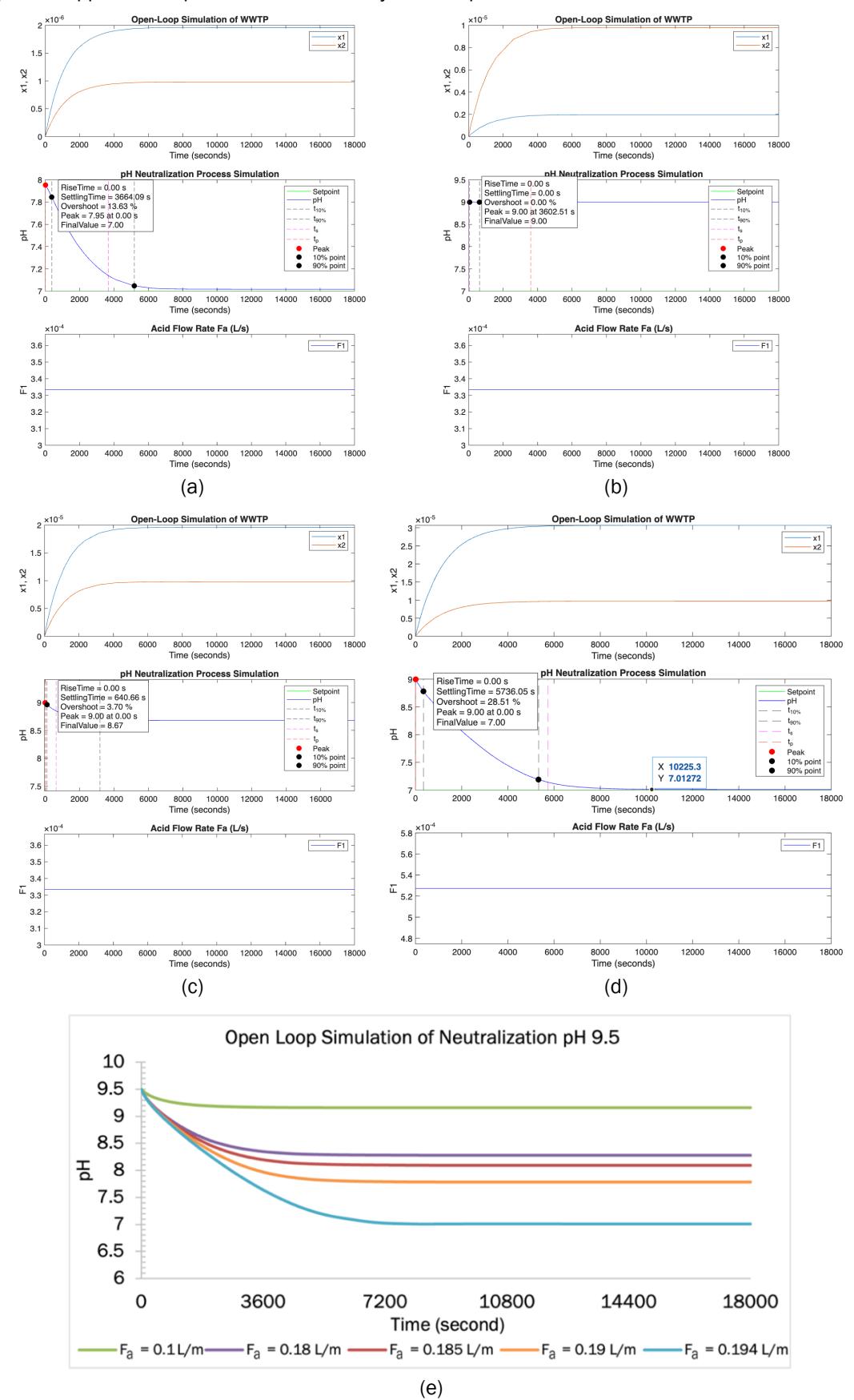
Figure 4. Open loop simulation results of pH neutralization process.
Open loop simulation is tested at several pH in range 6–12 to determine its effect on each parameter Fa, Fb, and Ca. Results from those simulations are then tabulated in Table 1.
Table 1. Open loop simulation parameters
| pH | Fa (L/min) | Fb (L/min) | Ca (M) | tss (s) | pHss | Transient time (s) |
|---|---|---|---|---|---|---|
| 12 | 2.677399 | 1 | 10 | 3496.34 | 7.21 | 3647.93 |
| 11.5 | 2.7010 | 1 | 1 | 3261.71 | 7.00 | 3424.12 |
| 11 | 2.7769 | 1 | 0.1 | 2833.39 | 7.03 | 3029.98 |
| 10.5 | 3.0343 | 1 | 0.01 | 2337.24 | 6.99 | 2551.45 |
| 10 | 0.14373 | 1 | 0.01 | 6838.64 | 7.01 | |
| 9.5 | 0.1940 | 1 | 0.001 | 5646.90 | 7.01 | 6636.43 |
| 9 | 0.03164 | 1 | 0.001 | 5643.73 | 7.01 | 7244.57 |
| 8.5 | 0.0757 | 1 | 0.0001 | 4350.02 | 7.03 | 6175.33 |
| 8 | 0.02002 | 1 | 0.0001 | 3526.56 | 7.01 | 5697.32 |
| 7.5 | 0.0501 | 1 | 0.00001 | 1436.06 | 7.00 | 4811.45 |
| 12 | 1.9117 | 0.7140 | 10 | 5019.39 | 7.07 | 5205.01 |
| 11.5 | 1.9285 | 0.7140 | 1 | 4567.09 | 7.02 | 4802.25 |
| 11 | 1.9827 | 0.7140 | 0.1 | 3923.47 | 7.03 | 4180.85 |
| 10.5 | 2.1662 | 0.7140 | 0.01 | 3230.19 | 7.03 | 3538.61 |
| 10 | 0.10263 | 0.7140 | 0.01 | 9623.65 | 7.00 | 10999.13 |
| 9.5 | 0.1385 | 0.7140 | 0.001 | 7852.59 | 7.02 | 9399.59 |
| 9 | 0.0226 | 0.7140 | 0.001 | 7983.36 | 6.99 | 9752.78 |
| 8.5 | 0.05412 | 0.7140 | 0.0001 | 6199.45 | 7.01 | 8737.08 |
| 8 | 0.01418 | 0.7140 | 0.0001 | 4665.30 | 7.06 | 7950.04 |
| 7.5 | 0.0358 | 0.7140 | 0.00001 | 2018.40 | 7.00 | 6351.24 |
| 9.5 | 0.1940 | 1 | 0.001 | 5646.90 | 7.01 | 6636.43 |
| 9.5 | 0.1467 | 0.7561 | 0.001 | 7518.93 | 7.00 | 8752.95 |
| 9.5 | 0.1455 | 0.75 | 0.001 | 7524.16 | 7.01 | 8829.10 |
| 9.5 | 0.14195 | 0.7318 | 0.001 | 7655.93 | 7.03 | 9175.20 |
| 9.5 | 0.1385 | 0.7140 | 0.001 | 7852.59 | 7.02 | 9399.59 |
| 9.4 | 0.0926 | 0.7140 | 0.001 | 8070.11 | 7.01 | 9624.61 |
| 9.32 | 0.06824 | 0.7140 | 0.001 | 8167.95 | 6.99 | 9739.23 |
| 9.2 | 0.04419 | 0.7140 | 0.001 | 8101.25 | 6.99 | 9749.17 |
| 9.19 | 0.04265 | 0.7140 | 0.001 | 7926.75 | 7.02 | 9865.86 |
| 9.15 | 0.03715 | 0.7140 | 0.001 | 8025.48 | 7.00 | 10001.65 |
| 9.1 | 0.03136 | 0.7140 | 0.001 | 7999.16 | 6.99 | 10026.60 |
| 9.05 | 0.02657 | 0.7140 | 0.001 | 7880.46 | 7.00 | 9890.96 |
| 9 | 0.0226 | 0.7140 | 0.001 | 7983.36 | 6.99 | 9752.78 |
The open-loop simulation results serve as a baseline for defining performance criteria in the subsequent PI and nonlinear adaptive control design for the pH neutralization process. As summarized in Table 1, two
operating scenarios are evaluated: the wastewater flow rate (Fb) is held constant at either 1 L/min or 0.7140 L/min within each scenario, while the neutralizer concentration (Ca) is adjusted according to the influent pH. Based on the open-loop response characteristics, several key observations can be made:
- 1. For the same influent pH and the same Ca, increasing the wastewater flow rate from 0.7140 to 1 L/min generally requires a higher neutralizer flow rate (Fa) to maintain the outlet near the neutral region.
- 2. In many cases, the response at Fb = 1 L/min reaches steady state faster than at Fb = 0.7140 L/min, as indicated by smaller settling time (tss) and, where reported, shorter transient time.
- 3. At a fixed Fb, increasing the influent pH in the highly alkaline region (approximately pH 10.5–12) requires a substantial increase in the neutralizer concentration Ca. Accordingly, Ca increases by about one order of magnitude (10×) for each 0.5 pH increment, equivalent to roughly 100× per 1 pH, reflecting the nonlinear nature of the neutralization chemistry.
- 4. At most operating points, the steady-state outlet pH (pHss) remains close to neutral (around pH 7). However, under extreme influent conditions (e.g., pH 12), a larger steady-state deviation can still be observed.
- 5. Even under the same Fb condition, tss and, where available, transient time can vary non-monotonically with influent pH, indicating that a smaller deviation in operating point does not necessarily imply a faster openloop convergence.
Although the neutralizer concentration (Ca) can be varied in the simulation, changing Ca is typically impractical in real WWTP operation because the plant usually relies on a single neutralizer storage tank. Therefore, Ca is assumed constant for implementation, and the manipulated variable is the neutralizer flow rate (Fa).
Furthermore, Figure 5 shows that the larger neutralizer concentration (Ca) causes smaller pH value, this is because neutralizer used is weak acid.
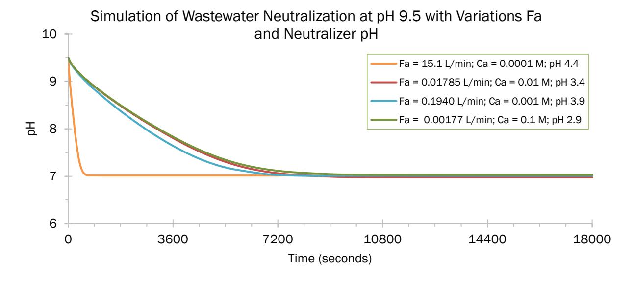
Figure 5. Simulation results of wastewater pH 9.5 neutralization by varying flow rate and neutralizer pH.
Economically, it might be more profitable to use neutralizer with pH 4.4 but requires quite large neutralizer flow rate and exceeds pump capability used in implementation stage. Therefore, in pH neutralization process implementation, acetic acid neutralizer solution with concentration 0.01 M and pH 3 is used, so pump can flow neutralizer according to pump capability.
3.2 Closed Loop PI Simulation
Based on open loop system response and PI Ziegler Nichols tuning results, parameter values Kp = −5.8121×10⁻⁵ and Ki = −2.4251×10⁻² are obtained. Therefore, in this PI simulation, Kp and Ki with those values are used. Furthermore, system linearity can be determined by observing time constant T, gain K, and dead time L from each wastewater. Flow rate and neutralizer concentration parameters used for closed loop PI simulation can be seen in Table 2.
Table 2. Closed loop PI simulation parameters
| Simulation Parameter | PI parameter | ||||||||
|---|---|---|---|---|---|---|---|---|---|
| рН | Fa (L/min) | Fb (L/min) | Ca (M) | tss t(s) | \[pH_{ss}\] | Т | K | L | Ti |
| 7.5 | 0.0501 | 1 | 0.00001 | 4865 | 7.00 | 1260 | -401.7 | 124.5 | 5040 |
| 8 | 0.02002 | 1 | 0.0001 | 3336 | 6.99 | 1852 | -2830 | 94 | 22228 |
| 8.1 | 0.026 | 1 | 0.0001 | 3643 | 6.99 | 2104 | -2450 | 91 | 27351 |
| 8.2 | 0.0338 | 1 | 0.0001 | 3838 | 6.98 | 2170 | -2097 | 88 | 30377 |
| 8.3 | 0.044 | 1 | 0.0001 | 4121 | 6.98 | 2229 | -1750 | 42 | 34555 |
| 8.4 | 0.0575 | 1 | 0.0001 | 4776 | 6.99 | 2384 | -1427 | 41 | 36947 |
| 8.5 | 0.0757 | 1 | 0.0001 | 4772 | 7.00 | 2345 | -1153 | 40 | 37526 |
| 8.6 | 0.1009 | 1 | 0.0001 | 4660 | 6.97 | 2484 | -958 | 38 | 37886 |
| 8.7 | 0.1355 | 1 | 0.0001 | 4527 | 7.00 | 2388 | -741 | 37 | 38205 |
| 8.8 | 0.1852 | 1 | 0.0001 | 4849 | 6.99 | 2433 | -583 | 32 | 38921 |
| 8.9 | 0.258 | 1 | 0.0001 | 5067 | 6.98 | 2354 | -444 | 25 | 40026 |
| 8.5 | 0.00734 | 1 | 0.001 | 1359 | 6.99 | 2588 | -12233 | 41 | 36226 |
| 8.6 | 0.00966 | 1 | 0.001 | 1398 | 6.99 | 2649 | -10061 | 40 | 37088 |
| 8.7 | 0.01278 | 1 | 0.001 | 1680 | 6.98 | 2690 | -7866 | 38 | 37667 |
| 8.8 | 0.01711 | 1 | 0.001 | 1735 | 6.99 | 2713 | -6339 | 36 | 40693 |
| 8.9 | 0.02312 | 1 | 0.001 | 2061 | 6.98 | 2687 | -4904 | 29 | 42990 |
| 7.5 | 0.0358 | 0.714 | 0.00001 | 4996 | 7.00 | 2077.7 | -564.4 | 144.2 | 6233 |
| 8 | 0.01418 | 0.714 | 0.0001 | 4057 | 7.00 | 2906 | -3772 | 113 | 23245 |
| 8.1 | 0.01851 | 0.714 | 0.0001 | 3995 | 7.00 | 3027 | -3360 | 108 | 30265 |
| 8.2 | 0.0234989 | 0.714 | 0.0001 | 5521 | 7.07 | 2549 | -2436 | 106 | 35680 |
| 8.3 | 0.0308594 | 0.714 | 0.0001 | 6331 | 7.06 | 2932 | -2120 | 101 | 46914 |
| 8.4 | 0.0411 | 0.714 | 0.0001 | 4959 | 6.99 | 3382 | -2022 | 96 | 54110 |
| 8.5 | 0.05412 | 0.714 | 0.0001 | 5169 | 7.00 | 3314 | -1640 | 92 | 56341 |
| 8.6 | 0.072 | 0.714 | 0.0001 | 5482 | 6.99 | 3378 | -1331 | 44 | 60806 |
| 8.7 | 0.0969 | 0.714 | 0.0001 | 5530 | 6.99 | 3470 | -1063 | 43 | 64191 |
| 8.8 | 0.1322 | 0.714 | 0.0001 | 6310 | 7.00 | 3357 | -813 | 41 | 65470 |
| 8.9 | 0.1842 | 0.714 | 0.0001 | 6251 | 7.00 | 3296 | -621 | 36 | 65926 |
| 8.9 | 0.01651 | 0.714 | 0.001 | 2449 | 6.98 | 3762 | -6888 | 41 | 75241 |
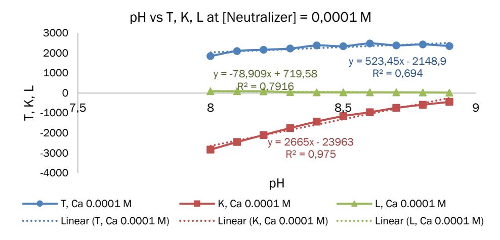
Figure 6. Relationship between pH and T, K, L at neutralizing agent concentration of 0.0001 M
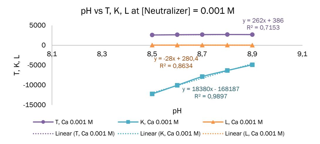
Figure 7. Relationship between pH and T, K, L at neutralizing agent concentration of 0.001 M
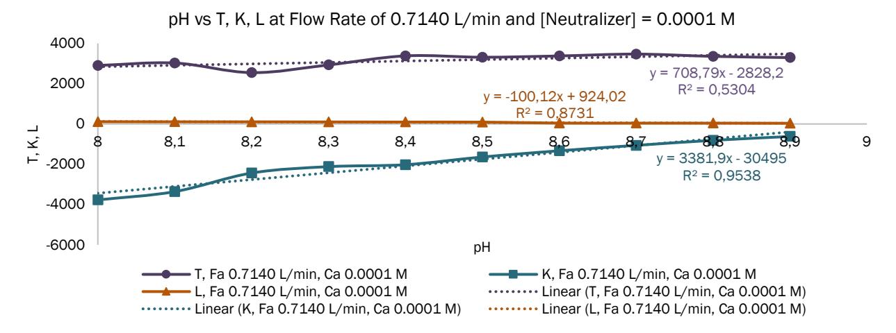
Figure 8. Relationship between pH and parameters T, K, L at flow rate of 0.0119 L/s and neutralizing agent concentration of 0.0001 M.
Based on data in Table 2 and T, K, L graphs in Figures 6-8, several things can be concluded:
- 1. At the same \(F_b\) and \(C_a\), the larger initial wastewater pH, the larger time constant and gain, but dead time becomes smaller.
- 2. Largest T and K regression results at \(F_b = 1\) L/min and \(C_a = 0.001\) M are 0.72 and 0.99. Meanwhile, largest L regression result at \(F_b = 0.7140\) L/min and \(C_a = 0.0001\) M is 0.87. From these regression results, it's concluded that wastewater approaches linear values with pH 8 to 8.9.
Figure 9 is one example of closed loop PI simulation results with parameters \(K_p = -5.8121 \times 10^{-5}\) and \(T_i = 8.4715 \times 10^{7}\). Meanwhile, wastewater parameters are pH 9, \(F_a = 0.03164\) L/min, \(F_b = 1\) L/min and \(C_a = 0.001\) M. With those parameters, open loop system response can reach steady state in 10225 seconds at pH 7.01. Meanwhile, closed loop PI response can reach setpoint 7 in shorter time, namely 3080.96 seconds.
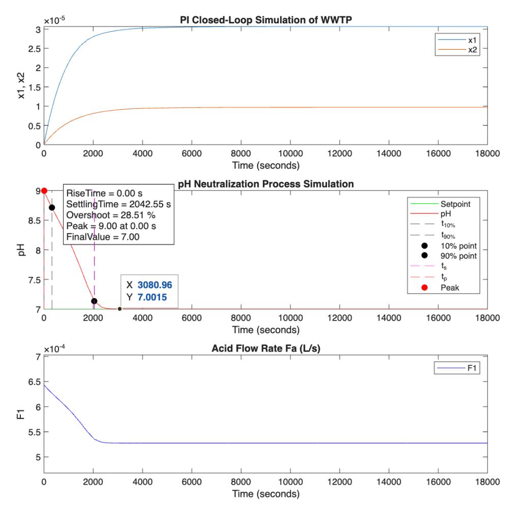
Figure 9. Closed loop PI simulation results.
3.3 Closed Loop Adaptive Simulation
In pH neutralization process simulation conducted by Sankar De et al. with giving k>0, \(\gamma_1>0\), \(\gamma_2>0\) neutralization process stability can be guaranteed. In this simulation, adaptive control of pH neutralization process uses controller parameter values k=8, \(\gamma_1=20\), dan \(\gamma_2=40\), producing closed loop adaptive controller simulation graph as in Figure 10. Wastewater parameters given are pH 9, \(F_a=0.03164\) L/min, \(F_b=1\) L/min and \(C_a=0.001\) M. With those parameters, closed loop adaptive control system response can reach setpoint 7 in shorter time than open loop or PI response, namely 2488.68 seconds.
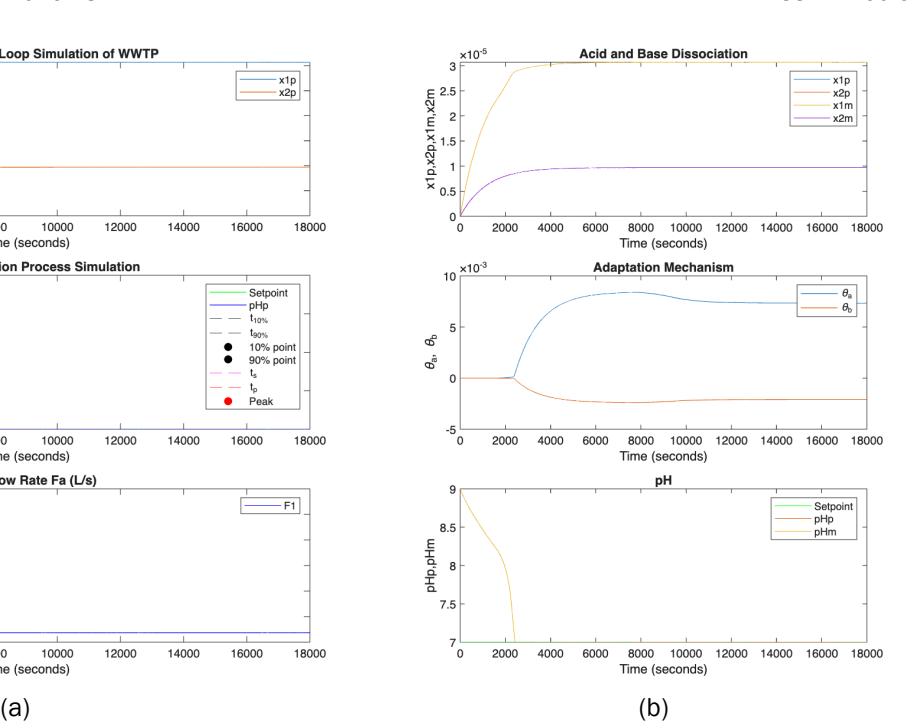
Figure 10. Closed loop adaptive simulation results.
3.4 Discussion
Closed-loop control using the PI controller and the nonlinear adaptive controller was evaluated for regulating the pH neutralization process to the setpoint (sp = 7), and the key results are summarized in Table 3. All evaluation metrics discussed in this section follow the definitions provided in Section 2.3.4. Both controllers satisfy the safety requirement against over-acidification because the minimum outlet pH remains above the lower bound (LimitLow = 6.80). This is confirmed by the minimum pH values, (pHmin = 7.0019) for the detuned PI controller and (pHmin = 7.0000) for the MRAC controller, indicating that neither strategy drives the process into an undesired acidic region under the tested scenario. For pH neutralization, constraint-based indicators such as (LimitLow) and (pHmin) provide a more meaningful safety assessment than the standard step-response "Overshoot" metric, because the regulated response corresponds to a downward transition (from pH 9 to 7) and the conventional overshoot definition does not directly represent lower-bound violations.
In terms of tracking accuracy, the PI controller outperforms MRAC based on the integral error indices. The PI controller yields IAE = 2774.85 and ISE = 3611.74, whereas MRAC yields IAE = 3199.85 and ISE = 4692.61, indicating that PI maintains smaller cumulative deviations from the setpoint over the simulation horizon. In contrast, MRAC achieves faster convergence, as reflected by the shorter settling time of 2377 s compared with 2566.4 s for PI. These results therefore reveal a clear tradeoff in which the "faster" MRAC configuration improves settling behavior but increases the integrated tracking error under this operating condition. Further tuning is thus recommended so that MRAC can preserve the faster settling time while reducing IAE or ISE.
From an operational perspective, chemical usage is quantified by the total injected neutralizer volume. MRAC consumes 9.5380 L compared with 9.5969 L for the PI controller, corresponding to an approximately 0.61% reduction. This small decrease is reflected in the composite cost, with MRAC yielding a slightly lower value of J=0.9939 than PI with J=1.0000. Because the lower pH bound is never violated, the safety-penalty term remains inactive, and the difference in J is therefore dominated by the neutralizer-consumption component. Overall, these results indicate a practical tradeoff in which MRAC provides faster convergence with marginally lower chemical usage and cost, whereas PI delivers better tracking accuracy as indicated by lower IAE and ISE. For practical deployment, MRAC implementations typically require additional safeguards beyond simulation tuning, such as parameter projection or bounding, σ-modification to mitigate parameter drift, and explicit actuator saturation handling (with anti-windup) to ensure realistic and stable control actions under changing influent characteristics or stronger disturbances.
Table 3. Comparison results of PI and adaptive controllers
| Category | Parameters/metrics | PI controller | Adaptive controller | |
|---|---|---|---|---|
| Controller parameters | Kp | -3.7778×10⁻⁵ | - | |
| Ki | -1.3338×10⁻² | - | ||
| Ti | 8.4715×10⁷ | - | ||
| K | - | 8 | ||
| γ1 | - | 20 | ||
| γ2 | - | 40 | ||
| Error indices | IAE | 2774.85 | 3199.85 | |
| ISE | 3611.74 | 4692.61 | ||
| Tradeoff result | J (Cost function) | 1.0000 | 0.9939 | |
| Min pH | 7.0019 | 7.0000 | ||
| Neutralizer (L) | 9.5969 | 9.5380 | ||
| Time-domain metric | SettlingTime (s) | 2566.39 | 2377.03 | |
4 Conclusion
This research successfully designed and evaluated an automatic control system for batik wastewater pH neutralization in a laboratory-scale WWTP (87.75 l) by comparing PI and MRAC controllers. Simulation results reveal a clear tradeoff where PI provides better tracking accuracy (IAE = 2774.85; ISE = 3611.74) but has slower settling time (2566.4 s) and higher neutralizer consumption (9.5969 L). Conversely, Adaptive MRAC achieves 7.4% faster response (2377 s), saves 0.61% neutralizer consumption (9.5380 L), and reduces the composite cost function (J = 0.9939), despite larger tracking error (IAE = 3199.85; ISE = 4692.61). Both controllers meet safety criteria by maintaining minimum pH above the lower bound of 6.80 (pHmin PI = 7.0019; MRAC = 7.0000) and keeping outlet pH within the quality standard range (pH 6–9) according to Minister of Environment and Forestry Regulation No. P.16/MENLHK/SETJEN/KUM.1/4/2019 (second amendment to Minister of Environment Regulation No. 5 of 2014). Therefore, controller selection depends on operational priorities with PI recommended for high accuracy or MRAC for faster response and neutralizer consumption efficiency with adequate implementation safeguards.
Acknowledgement
The authors acknowledge the ITB Excellence Research Program 2022, which funds this research.
Nomenclature
Chemical Constants
ka = Acid dissociation constant
kb = Base dissociation constant
kw = Water dissociation constant (1×10–14 at 25°C)
Process Variables
Fa = Acid neutralizer flow rate, L/min
Fb = Wastewater flow rate, L/min
Ca = Acid neutralizer concentration, M (mol/L)
Cb = Wastewater concentration, M (mol/L)
Vt = Final tank volume (or Tank volume), L
t = Time
pH = Degree of acidity
State Variables
x1 = Acid dissociation, mol/L
x2 = Base dissociation, mol/L
xp = Combined dissociation state ( x1 − x2), mol/L
xm = Reference model state, mol/L
Chemical Species
CH3COOH = Acetic acid (weak acid)
CH3COO− = Acetate ion (conjugate base)
NaOH = Sodium hydroxide (strong base)
Na+ = Sodium ion
H+ = Hydrogen ion
OH− = Hydroxide ion
H2O = Water
Control Variables
r = Bounded reference input (pH setpoint)
e = Error signal (e = xp − xm)
u = Control signal (neutralizer flow rate), L/s θa = Adaptive parameter a θb = Adaptive parameter b
Controller Parameters
Kp = Proportional gain (PI controller)
Ki = Integral gain (PI controller)
Ti = Integral time constant, s
1 = Adaptation gain 1 (MRAC)
2 = Adaptation gain 2 (MRAC)
k = Controller parameter (MRAC)
Performance Metrics
T = Time constant, s
K = System gain
L = Dead time (time delay), s
tss = Settling time (steady-state time), s
pHss = Steady-state pH value
= pH safety margin for lower bound, pH
LimitLow = Lower pH limit
VN = Total neutralizer volume, L IAE = Integral of absolute error ISE = Integral of squared error
J = Composite cost function (tradeoff index)
Jos = Acid-undershoot penalty term
Ju = Neutralizer usage term (often = V)
Jos,n = Normalized acid-undershoot penalty
Ju,n = Normalized neutralizer usage
Mathematical Functions
V = Lyapunov function candidate
V̇ = Time derivative of Lyapunov function
Subscripts
a = Acid
b = Base/wastewater
w = Water
t = Tank
m = Model (reference)
n = Normalized
N = Neutralizer
p = Process
os = Acid-undershoot
ss = Steady state
0 = Initial condition