

I. INTRODUCTION
1.1 Background
It is well-known that there is a very close relationship between the provision of transportation system infrastructure and the development of urban structure and land use. Given the current worldwide transportation problems such as increasing traffic congestion and energy crises, there is a fast growing interest within large conurbations in developing countries in providing public transport in effective and efficient forms such as mass transit systems (Fouracre et al. 1990).
However, the success of the adoption of mass transit is also influenced by, and results from, a good planning stage as well. It can be argued that the selection of the system to be adopted is also dependent on the demand modelling method used in the preparation of the proposal, especially related to the prediction of the transport demand level and the capacity of the system which is required to accommodate it. Allport and Thomson (1990) reported that the performance of some new mass transit system in developing cities was unsatisfactory
due to the mistakes made in the planning stages, such as patronage overestimates.
Jakarta, which has been suffering for many years with similar transportation problems to other large developing cities due the very rapid economic development which increase the demand for the movement of people and goods, which then cannot be accommodated on the existing transportation system, has conducted many studies in order to find effective and affordable solutions such as The Jabotabek Railway Development Master Plan (JRDMP) in 1982. The Arterial Road System Development Study (ARSDS) in 1987, The Integrated Transportation System Improvement (ITSI) in 1990, The Transportation Network Planning and Regulation (TNPR) and The Jakarta Mass Transit System (JMTS), all in 1992.
Of the studies mentioned above, three (ITSI, TNPR and JMTS) had similar objectives and were carried out at almost the same time, using the same basic data sources. However they presented proposals that differed substantially from each other. All three studies adopted different methodologies, which resulted in different socio-economic and trip demand forecasts, and recommended alternative networks and corridors for development, as well as the proposed technology to be adopted, as shown in Figure 1.1. Thus, the ITSI study proposed a system that relied mainly on heavy rail technology in combination with other still undefined modes (but probably light rail transit), the TNPR study proposed a system that combined bus ways with both heavy and light rail, while the JMTS study proposed a combined system of light and heavy rail technologies.
Using this situation as a case study, this work intends to compare and assess the suitability of the models used in each of the proposals in the context of a developing country such as Indonesia. Each study team adopted transport planning methods originally developed and commonly used in the developed world. Therefore, the appropriateness of the application of these methods to a developing city like Jakarta can also be assessed, bearing in mind that dissimilar conditions in different countries could lead to unsuitable models being adopted, unless they are modified or simplified.
1.2 Work program
In order to achieve the research objectives, the following work program was set up:
- Review the three studies and their methodologies to seek explanations for the divergences which occurred in terms of the methods or models used and the forecasting of results.
- Compare the methods and the results of the three studies based on both theoretical and practical application points of view, using a descriptive and qualitative analysis framework. Also, more recent data and information are used for comparison.
- Draw conclusions and recommendations which could be used as lessons for the future in other cities in Indonesia or elsewhere.
Source: Jakarta Public Mass Transit System
Figure 1.1 Alternative network proposals
1.3 Data and limitations
The data used for this research consists of primary data (obtained from surveys or direct observation in the field) and secondary data (obtained from the original proposals and other relevant studies or reports, and from computer data files used in JMTS and TNPR).
Due to difficulties in obtaining all of the data required from the original studies or from the direct surveys, much of the work is based on data from just one of the studies which was then assumed to be valid for other studies as well.
II. REVIEW AND COMPARISON OF THE THREE STUDIES
2.1. The authorisation and terms of reference of the studies
Of the three particular studies concerned, ITSI was conducted under the direction of the Railway Authorities, whereas TNPR was executed under the direction of the Directorate of Urban Transportation. Finally JMTS was conducted under the direction of the Ministry of Research and Technology.
The detailed terms of reference of each study varied due to the different commissioning authorities and their different points of view and responsibilities. However, all three studies were instructed to recommend a system that should take into account, and be fully integrated with, the existing public transport system and the available infrastructure.
ITSI was carried out as the follow-up to the JRDMP in 1985, with the objective to formulate an Integrated Transportation System plan in the Jabotabek Area, to enhance the role of the railways and to provide links with road transportation and metropolitan development plans. TNPR was undertaken as a part of the Jabotabek Urban Development Project, with the special task to investigate
future levels of travel demand in and around the study area and identify an appropriate set of possible mass transit routes and services which could meet the requirement of forming a comprehensive integrated mass transit network. Finally, JMTS was conducted as a pre-feasibility study in order to propose a suitable system for a mass transit system in Jakarta based on an integrated network, and to identify a priority ranking of the projects to be investigated in more detail in a feasibility study.
2.2. Overview of the methodology of the studies
In terms of the whole planning process, the general structure of their methodologies can be represented as shown in Figure 2.1. The planning process started by reviewing the trip demand from the available ARSDS data and the result of surveys carried out in the studies, which was then updated and adjusted in accordance with the planning framework of the studies and the current socio-economic data. At the same time, an inventory was made of the existing transport network. This, in conjunction with the planning framework, was used in the trip demand modelling and in formulating strategies. Next, the pre-selected strategy options were fed into the trip modelling process to find the most suitable strategy to be recommended. This process was carried out iteratively. In an almost parallel work, the accompanying measures to ensure the success of implementing the strategy were also investigated and put into the demand modelling process (e.g. through the inclusion of traffic restraint in the model).
2.3 Planning framework
2.3.1. Horizon year
All three studies used different horizon years, although they all based on long term strategies of 20 - 30 years ahead. The horizon year in ITSI was 2005, in TNPR 2010 and in JMTS 2015. In this aspect, the shorter
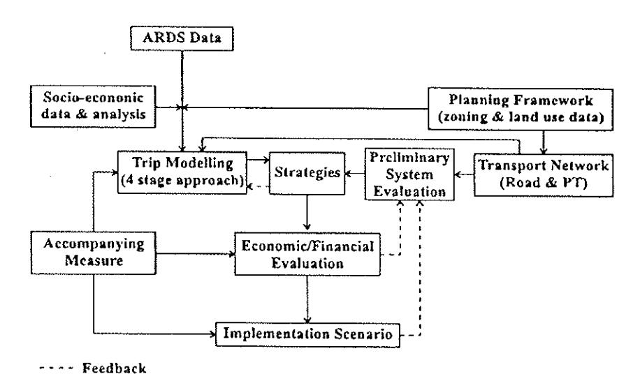
Figure 2.1 General methodological structure of the three studies
horizon in ITSI (less than 20 years) was perhaps due to the fact that it was essentially a continuation of the previous JICA study and might be followed by other studies.
2.3.2. Zoning system
The zoning system for all three studies were mainly based on administrative structures. The ITSI study used the old structure (before 1987), with 113 zones (90 for Jakarta and 23 for Botabek) based on villages, whereas TNPR and JMTS used the new structures with TNPR based on villages (190 zones, 146 for Jakarta and 44 for Botabek) and JMTS based on the sub-regencies (59, i.e. 42 for Jakarta and 17 for Botabek). The external boundaries in all studies were the same, but some internal zone boundaries were different, especially between ITSI's zones and the other two. Each JMTS zone consists of one or more TNPR zones, i.e. aggregated from village level into sub-regency level, thus they are both compatible. However, some of the ITSI zones are included in different JMTS or TNPR zones and the degree of overlap, between them is approximately 80%.
In this respect, ITSI's zone system would be more difficult to check against the current
situation and future developments. Therefore, its planning results would also be difficult to revise or adjust. The more detailed zone system used by TNPR might be better than the other two since it can give finer results; however, it needs more data and analysis as well as more complicated calculations or estimations. On the other hand, JMTS used a rather coarse zoning system based on sub-regencies in the new administrative structure, which has certain advantages due to its relative simple system. However, some of their intra-zonal trips could be lost due to the level of aggregation. However, this defect was partially overcome by using the TNPR zone system for fine tuning its demand model calibration.
For more advanced stages of the plan, a more detailed zone system would be required to model the strategy more precisely. For example, in the basic design stage, the number of zones used was 198 (see Halcrow Fox, 1996).
2.3.3 Urban structure, spatial distribution and land use development
All three studies based their approach to these aspects on the Jakarta and Jabotabek Master Plans. However, in their analysis
they emphasized different points to back up their development scenarios.
In ITSI, the conceptual population distribution up to 2005 was concentrated in areas to the west and east of Jakarta. A multicore structure with eight activity centres was proposed for work places, all to be developed around railway stations. Large and medium industries were to be located or relocated downstream of Jakarta, whilst small and home industries would be dispersed into neighboring residential areas. In TNPR, the future development scenarios defined by the Jakarta Masterplan 2005 were fully adopted, taking into account some rapid development in certain areas such as Blok M, Setia Budi (Golden triangle) and Kemayoran. According to JMTS, the rapid development of some areas in Jakarta would lead to a change of function from residential into business areas with consequent depopulation. In the Botabek region, the development would be restricted along the border of Botabek in the vicinity of each city. The differences in these assumptions led to different zone growth factors for example and, subsequently, different trip distribution patterns, as observed in the three studies.
2.4 Exogenous factors
2.4.1 Population
The population forecast from all three studies are shown in Figure 2.2 for Jakarta and Figure 2.3 for Jabotabek (some inter-mediate figures were extrapolated due to incomplete information obtained). They show that there are large differences about the predicted future populatio for Jakarta resulting from different data sources and development scenarios assumed. TNPR gave the highest predictions, and JMTS the lowest. However, for Jabotabek as a whole, the trend was almost the same except for ITSI which gave a lower growth rate.
The ITSI study based its population forecast on the 1987 Indonesia Statistical
Year Book and the 1981 Population census. In TNPR, the data sources used were Zonal registration data in 1985, the Jakarta Structure Plan evaluation team for 1987 and 1988 and the SUPAS (Intercensal) population total for 1985, and also the report of the study "The Demography of Jakarta in the 1980s". This last report gives forecasts to 2005 under various scenarios of fertility and migration. TNPR chose a low fertility and high migration scenario and extrapolated it to 2010. Forecast of the number of households in each zone were based on the 1988 average household size obtained from the Jakarta Evaluation Team estimates. These estimates were used with population estimates to obtain the estimated number of household by zone.
JMTS conducted its population study based on the census data from 1970, 1980 and 1990. In their analysis, partly based on past trends, three different scenarios were created, i.e. the best, middle and worst case scenarios. The middle case scenario, which was chosen for further analysis, is similar to the best scenario (i.e. based on the assumption that the family planning programme would be successful, that the in-migration to Jakarta would decline and that the out-migration from Jakarta to Botabek would increase) but fertility decline would be less rapid and the predicted migration flows were slightly different. JMTS then used different appropriate forecasting parameters for Jakarta and Botabek to consider the different development level of the capital and the surrounding area.
Looking at this condition, the differences in data sources and forecasting methods used made the predicted populations very different from each other. However, in terms of methodology, JMTS seems better than the other two since it developed its own more rigorous model, and was also partly based on, or checked by, the latest census of 1990. This study also has another strength in that it considered three different scenarios (best, middle and worst).
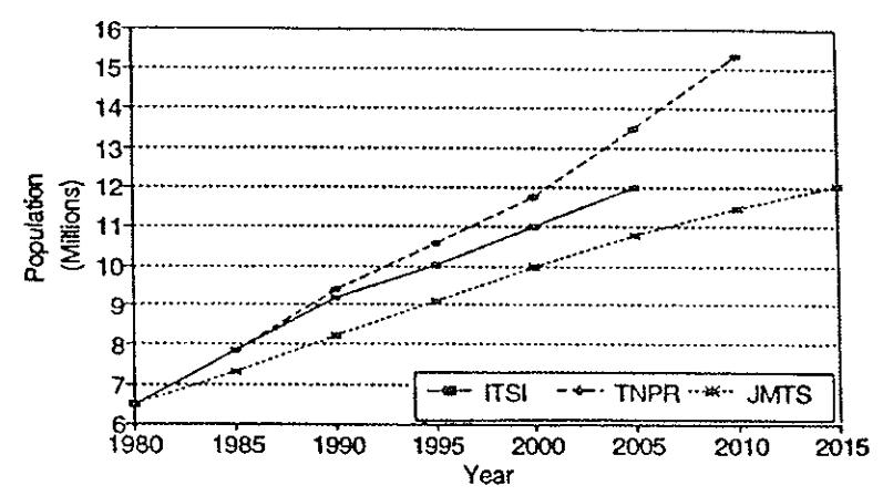
Figure 2.2 Population of Jakarta 1980 - 2015
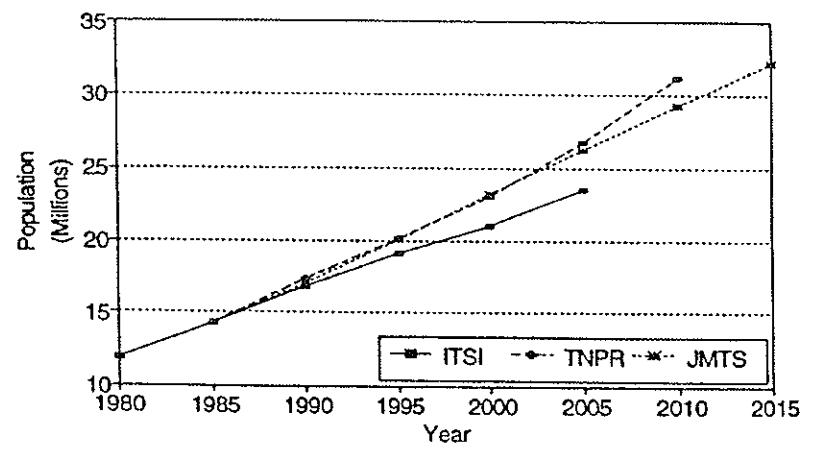
Figure 2.3 Population of Jabotabek 1980 – 2015
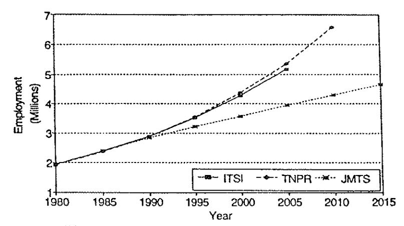
Figure 2.4 Employment in Jakarta 1980 - 2015
By contrast, the weaknesses of the other study methodologies were mainly in their basic procedure of following past trends obtained from forecasts of the Bureau of Statistics (in ITSI) or rather out-of-date
forecasts from the special study of the Demography of Jakarta in the 1980s report (in TNPR), without taking into account more recent developments such as the effect of family planning, migration trends etc.
2.4.2 Employment
The employment forecast from all three studies can be seen in Figure 2.4. It shows that ITSI and TNPR have a very similar trend, whereas JMTS gave a far lower predicted growth forecast.
According to ITSI, the labor force in Jakarta grew at an annual rate of 4.85% between 1980 and 1985. In TNPR, the number in employment in the base year (1985) was based on the SUPAS (intercensal) data for 1985. They represents an average annual predicted growth of 4.3%. In JMTS, the employment forecast was made by using a combination of two approaches, viz.: the labor force and economic approaches. The labor force approach was applied to analyze and forecast the total employment figures, whereas the economic approach assesses the total figures gained from the labor force approach and analyzes employment by specifying the role of the basic economic sectors.
In comparing of this aspect, JMTS seems to do better by combining two approaches into its forecasting method, whereas the other two studies mainly tended to use only economic trends. As a whole, based on the predicted future employment, it was found that TNPR again gave higher figures than the other two studies. To some extent this situation might simply be explained by the fact that a higher population ought to lead to more employment, although this is not always the case and there is another possibility of employees commuting in from other areas.
2.4.3 Income distribution
The analysis and forecast of income distribution, were carried out rather differently in each study. In ITSI, the analysis was based on household expenditure data obtained from the 1984 National Social Economic Survey (SUSENAS). In TNPR, the best available estimate of per capita expenditure for Jakarta for 1985 was also based on
SUSENAS in 1985. In JMTS, the income growth in Jakarta between 1980 - 2015 was estimated to be 2.7% p.a. The forecast distribution of income groups and their trend was predicted to change, with the percentage of low incomes decreasing and the percentage of high incomes in-reasing.
In this case, in ITSI, no further information was available about the forecasting of future income or expenditure, and this aspect was represented by economic development in terms of GRDP. On the contrary, the TNPR approach can be compared with JMTS, resulting in a general conclusion that based on the distribution of the population in various income groups, JMTS was more optimistic in predicting the percentage of population with a high income.
2.4.4 Vehicle ownership
Figures 2.5 and 2.6 show the forecast number of passenger cars and motorcycles in Jakarta from 1985 to 2015. For cars, TNPR had the highest growth rate. For motorcycles, ITSI predicted the highest number whereas the TNPR prediction increased from the lowest to almost the same as JMTS by 2010. It should be noted that the differences in the actual predicted numbers of vehicles were also caused by different starting points resulting from various data sources, which have divergent records of registered vehicles for unknown reasons.
In ITSI, using the Jakarta Masterplan 2005 report as its source, the ownership of private vehicles (passenger cars and motorcycles) was predicted to grow at a rate of 4 to 5% p.a. until 2005. The private vehicles was expected to reach the level of 2 million in year 2005. In TNPR no source of data was mentioned; however, the study considered that it was not possible to develop realistic model of vehicle ownership due to the poor data available. Therefore, it was decided to incorporate the joint effect of income and vehicle availability.
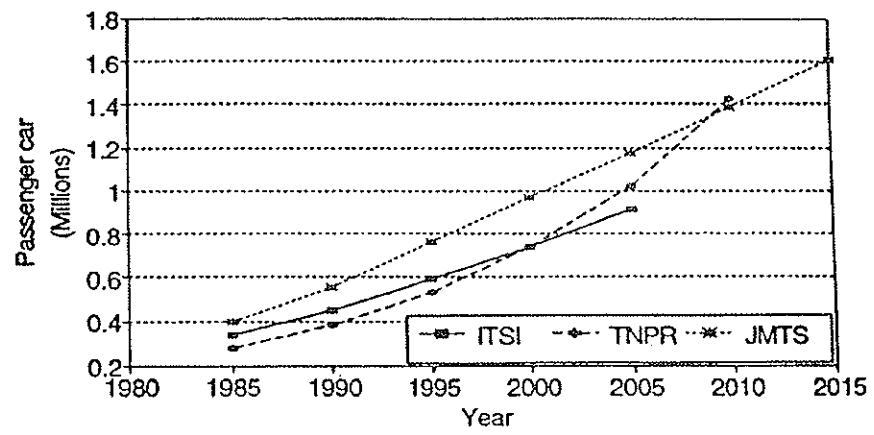
Figure 2.5 Number of passenger cars in Jakarta 1985 – 2015
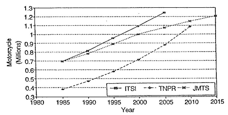
Figure 2.6 Number of motorcycles in Jakarta 1985 – 2015
The income distribution model was used to forecast the changing proportion of household with access to private vehicles. Then for the forecast year of 2010, the average proportion of household in each of the four vehicle availability groups, which was assumed constant over time, was distributed to forecast income groups. In JMTS, the study found that there was a very close correlation between the growth of the GRDP per capita and the growth of the number of passenger cars or motorcycles per thousand inhabitants. Therefore the prediction of vehicle ownership was based on the forecast of economic growth. In their forecast for the number of car in Jakarta, two scenarios (high and low) were adopted, the former being mainly based on current trends whereas the latter considered the capability of Jakarta to accommodate the maximum number of cars.
Looking at their methodologies, the JMTS study seem somewhat better. The forecast results in Figures 2.5 and 2.6 show that the TNPR scenario was the most optimistic in predicting a larger number of passenger cars and motorcycles in the future.
2.5 Comparison of forecast versus actual data factors
Based on the above analyses so far, the TNPR study always seems to give the highest predictions of exogenous factors to be used in the demand model. ITSI gave the lowest and JMTS stands in the middle. However, to check the accuracy of the forecast made by each study, the results of their forecast were compared with the data derived from in 1992, as shown in Table 2.1. These figures show that the predictions made by JMTS are closer to the actual data
Table 2.1 Forecast of the three studies versus actual data in 1992 (in '000)
| Aspect | Data 1992 | ITSI | TNPR | IMTS |
|---|---|---|---|---|
| Population | ||||
| - Jakarta | 7,309 | 9,600 | 10,000 | 8,600 |
| - Jabotabek | 15,493 | 17,100 | 17,300 | 17,200 |
| Employment | 3,145 | 3,100 | 3,100 | 3,000 |
| No. of Passenger Cars | 575 | 500 | 450 | 600 |
| No. of Motorcycles | 920 | 850 | 520 | 810 |
Note: The numbers for employment and vehicle ownership are for Jakarta only than the other two. However, the slightly worse results from ITSI could be caused by the prediction being made at an earlier time (i.e.in 1988 compared with JMTS in 1990).
In terms of population, the huge differences between the actual and forecast figures could yield a significant over-estimate in patronage. Moreover, it shows that the population in Jakarta tends to decrease rather than to increase as predicted and already detected in JMTS, who found that in 1990 the population of Jakarta was one million lower than the previous prediction (8.2 compared with 9.2 million). Also some zones have a lower population than before due to changes in land use from residential to business. On the other hand, the population of Botabek was higher than predicted. This clearly indicates that some of the former Jakarta population has now moved to the outskirt or to Botabek areas, although perhaps they still work in Jakarta; the commuter trips thus created will lead to a different pattern of trip distribution which will in turn affect the system required to accommodate these trips.
2.6 Trip demand modelling and analysis
2.6.1 Overview of works and models
In ITSI, the future transportation demand in the area was estimated sequentially as follows: trip matrix ARSDS 1985 update, model development and validation, and future demand forecast. Trips analyses and forecast in this study area comprise the trips within Jakarta, the trips between Jakarta and Botabek and the trips between Jakarta and other areas. Modes considered were railway, buses, a mass transit system, motorcycles and passenger cars. The first three modes were treated as a public mode, and the others as private mode. Trucks were considered as a freight transportation mode separate from the above modes.
In TNPR the network modelling was carried out using the MINITRAMP package and the trips were distinguished between internal (Jakarta) and external (Jakarta -Botabek). This study carried out the travel demand modelling for the first category, while the model from ARSDS was still used for the second. In JMTS the EMME/2 package was used for network modelling. The working steps for the study were data collection and processing, modelling Jabotabek 1990, and forecasting Jabotabek 2015. In modelling the demand O-D matrix, trips within Jakarta and trips between Jakarta-Botabek were separated. The internal Jakarta matrix for 1990 was derived from the ARSDS 1985 O-D matrix and adjusted to 1990. For the Botabek area, trip generation in Jakarta was adjusted by observing volumes on cordon counts.
2.6.2. Trip generation and attraction models
In ITSI, the trip generation and attraction models were estimated by using the 1985 ARSDS trip matrix and zonal population and employment parameters. There were five models, derived through regression analyses of the form:
\[G_i = A + B*E_i + C*P_i\] [2.1] where:
\(G_i\) = Daily trips generated/ attracted from or to zone i.
\(E_i = Employment of zone i.\)
\(P_i\) = Population of zone i.
In TNPR, internal Jakarta trips were developed through the use of regression models which depend on household type (segmented by 4 income groups and 4 vehicle availabilities). Trip purposes were distinguished as Home Based (HB), i.e. work, education and others, and Non Home Based (NHB), i.e. zone based generation. Only one-way HB or NHB (origin zone) trips were estimated and matrix manipulation was used to create return journeys. HB trips were developed as a function of household size and structure (number of employed and unemployed adults or housewives etc.) using simple linear equations unconstrained through the origin. On the other hand, the NHB trips were developed using the simple linear independent variables of employment and population density. For HB purposes, there were 48 separate models viz.: 4 income group * 4 vehicle availability group * 3 modes used (MC, PC and PT).
An example of the HB model was, for Work:
Thm = 0.314 * Empad. [2.2]
whereas for NHB the model was:
Thz = 0.394 * Emp + 0.05 * Popdens. [2.3] where:
Thm = Dr y trips per household for income group 1, vehicle availabinity group I and for mode
public transport.
Empad = Intender of employed adult.
Thz = Dail trips per zone. Emp = Zon-1 employment. Popdens = Zonal population density.
In JMTS, the factors selected for analyzing demand generated were: population, sectoral employment, land use and vehicle ownership. The forecast parameters were distinguished between Jakarta and Botabek. To include land use aspects, the total number of zones was divided into three classes. described by the ratio of population to the total number of relevant workplaces, which were:
- Class 1: employment-oriented areas (0-3 inhabitants per workplace).
- Class 2: mixed areas (3-5 inhabitants per workplace).
- Class 3: residential areas ( > 5 inhabitants per workplace).
Finally, based on multilinear regression, the general equation used for both generation and attraction was:
\[T_i = A + B*Pop_i + C*Wp_{iii}\] [2.4] where:
Ti = Total number of daily generated/attracted t rip of zones
= Population of zone i. \(Pop_1\)
= Total number of relevant \(Wp_{i \, iii}\)workplaces (sector iii) in zone i.
Comparing this aspect, the first drawback of the ITSI study occurred in its trip generation and attraction models, which used zonal population and employment as explanatory parameters. This could be considered as a slightly coarse approach, although it does have the advantage of simplicity. In TNPR, the trip production model used was based on household, which has the advantage of being more disaggregate and accounts for the trip purposes; therefore it was potentially more accurate as well. However, as a consequence, it needs more complicated data and analysis, and it is also more difficult to crosscheck. In JMTS, the models used for trip production were based on zonal parameters, as in the ITSI study; therefore, these models are also considered to be slightly weak.
On the other part, the total number of daily trips forecast in all three studies is shown in Figure 2.8. It is clear from this figure that JMTS gives the highest prediction, whereas
TNPR, which was almost similar to ITSI up to 1995, then becomes the lowest prediction of the three. Therefore, from this case study, it is clear that a higher prediction of exogenous factors does not necessarily lead to a higher trip demand prediction.
Having looked at the results, the demand forecast were clearly different given the different assumptions about the planning and socio-economic frameworks mentioned previously. To illustrate these differences, Figure 2.9 compares the trip generation results obtained by inputting the JMTS zonal population and employment data into both the ITSI and JMTS models. Figure 2.10 does the same but using the ITSI data.
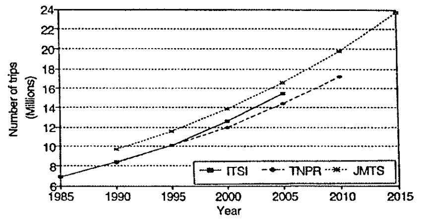
Figure 2.8 Number of total trips 1985 - 2015
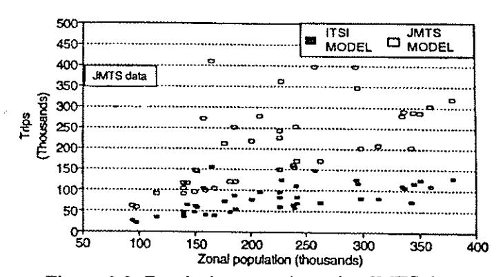
Figure 2.9 Zonal trip generation using JMTS data
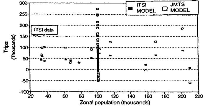
Figure 2.10 Zonal trip generation using ITSI data
These figures show that the trips produced by the JMTS models are always higher than the ITSI models. These figures also show that the use of ITSI data gives more scattered results, which might indicate some doubt over the model's validation and calibration process. Also, the distribution of ITSI zonal population data is mostly in the region of approximately 100,000. In addition, putting the ITSI data into the models can result in some negative trips which could be neglected or set to zero.
2.6.3 Trip distribution models
In ITSI, a trip distribution model was estimated from the O-D trip matrices and the road distances between zones. A gravity model was adopted to represent a daily one-way trip distribution pattern within the area and this model was estimated through a regression analysis as:
\[T_{ij} = 0.0001695 * G_i^{-0.7025} * A_j^{-0.70169} * d_{ij} - 0.26177\] [2.7] where:
\(T_{ij}\) = Trips between zones i and j
G<sub>1</sub> = Trips generated from zone i
A<sub>j</sub> = Trips attracted to zone j.
d<sub>ij</sub> = Road distance between zones i and j. (calculated through a minimum path algorithm based on the 1988 road network).
In TNPR, three approaches to trip distribution and mode choice were tried: conventional individual choice modelling, stated preference, and joint trip distribution-modal split (dual mode gravity model). The last model was finally selected because it produced the best results. According to TNPR, the dual-mode gravity model is an extended version of the simple gravity model, with trips from vehicle available-household jointly distributed between public and private modes, and trips from vehicle unavailable households constrained to public transport. The general form of model is as follows:
\[T_{ij}^{kn} = A_i^n O_i^n B_j D_j \exp(-\beta_n K_{ij}^n) \{ \exp(-\lambda_n C_{ij}^k) / \Sigma_k \exp(-\lambda_n C_{ij}^k) \}\] [2.8] where:
T<sub>ij</sub><sup>kn</sup> = Trip between i and j by mode k and by person type
\(A_i^n\) and \(B_j\) = Balancing factors.
O<sub>i</sub><sup>n</sup> and D<sub>j</sub> = Number of trips originating from O and destined to D.
C<sub>ij</sub><sup>k</sup> = Generalised cost of travel between zones i and j by
\(K_{ij}^{n}\) mode k. \(= \sum_{i} P_{ij}^{n} C_{ij} = Composite\)generalised cost for per-
\(P_{ij}^{n}\) son type n. = Proportion of trip using
mode k.
\(\beta_n\) and \(\lambda_n\) = Calibration parameters.
The model used by JMTS was the Fratar method (zonal growth factor). This method used a successive approximation approach to break down the total trip production of each traffic zone into interzonal volumes according to the following formula:
\[\begin{array}{l} {M_{ij}}^{N+1} = {M_{ij}}^{N-*} \ (g_i + a_j)/2 \ - \ G_i^{\ 1990}/{\sum_k}^n \ M_{ik^*ak} \ ^* \\ {A_j}^{\ 1990}/{\sum_k}^n \ M_{kj^*gk} \end{array}\]
[2.9] where:
\(M_{ij}^{N+1}\) = O-D matrix of motorised traffic after N+1 iterations.
M<sub>ij</sub> = Motorised traffic from zone k to j.
G<sub>i</sub><sup>1990</sup> = Total motorised traffic (tmt) generated by zone i in 1990 obtained by the formula derived from the regression analysis.
A<sub>j</sub> = Corresponding figure of tmt attracted by zone j in 1990.
\(g_i = G_i^{1990} / G_i^{n}\) \(= A_j^{1990} / A_j^{n}\)
n = Number of zones.
In this aspect, the use of a gravity model based on trip generated and attracted and road distance between O-D pairs, estimated through the regression analysis in the ITSI study, seems to be not a very advanced approach. The use of a dual-mode gravity model in TNPR has similar problems to that study's trip production models. For JMTS, the use of a quite simple growth factor method is also considered to be weak for a long term study, since it is usually more suitable for short term forecasting where no major development takes place in the area.
We may also compare the results of the trip distribution models among the three studies through the pattern of trip movements among O-D pairs. This is demonstrated, either in terms of total daily trips in 2005 from ITSI and JMTS (Figures 2.11 and 2.12), or in the peak hour trips in 2010 from the TNPR (Figure 2.13).
2.6.4 Modal split models
In ITSI, the modal split was combined with trip assignment and its model, which divides public trip into railway and bus modes, was estimated on the basis of the observed 1985 modal shares and explanatory variables derived from the 1988 networks. A time value mode split model was used; it deals with the two factors, time and cost of travel, which are then converted into the total generalised cost. This model assumes that the time value is a logarithmic normally distributed from experience. The complete equation can be seen below (equations 2.10 and 2.11).
In \[\lambda\] \[S2 = \int f(\ln \lambda) \cdot d\ln \lambda \qquad [2.10]\] \[f(\ln \lambda) = \frac{1}{\sqrt{2\pi\sigma \ln \lambda 2}} e^{-(\ln \lambda \cdot -\mu \ln \lambda) 2/2 (\sigma \ln \lambda) 2} \qquad [2.11]\] where: \[S2 = \text{modal share of the second mode; } \lambda = -(k1 - k2) / (t1 - t2)\] \[ki = \text{monetary cost by mode I; } t_i = \text{travel time by mode i}\] \[\mu \ln \lambda = \text{mean of } \ln \lambda; \quad \sigma \ln \lambda = \text{standard deviation of } \ln \lambda\]
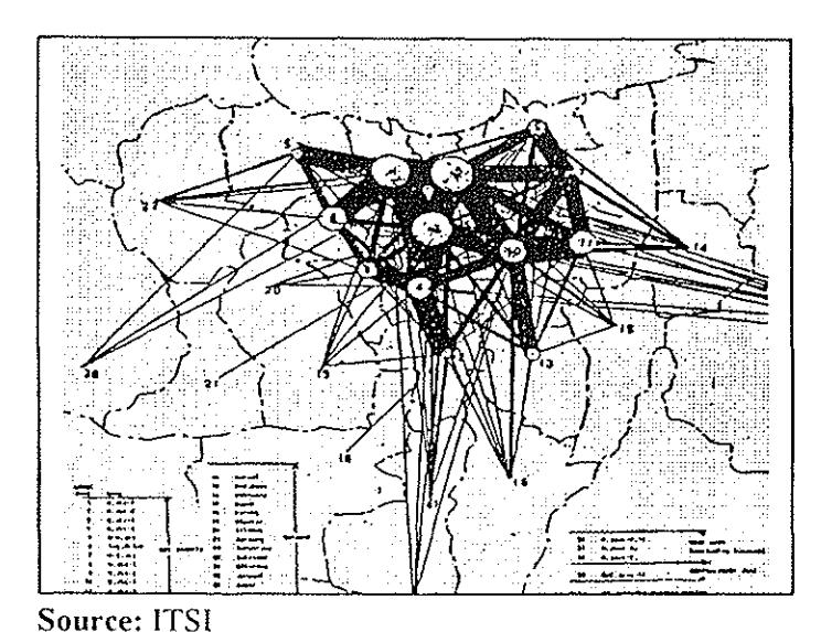
Figure 2.11. Daily trip movement pattern of ITSI in 2005
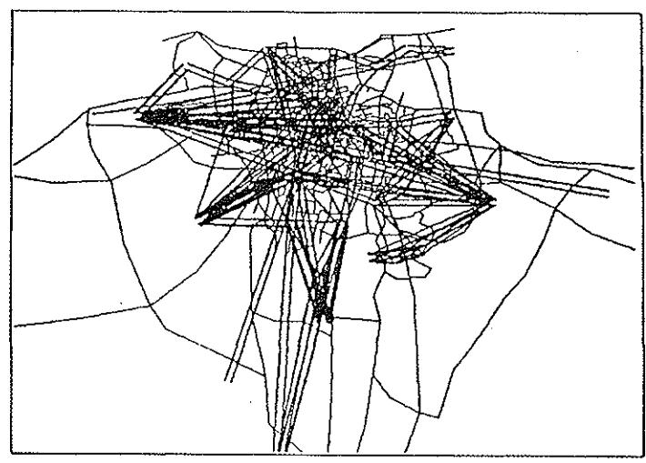
Figure 2.12. Daily trip movement pattern of JMTS in 2005
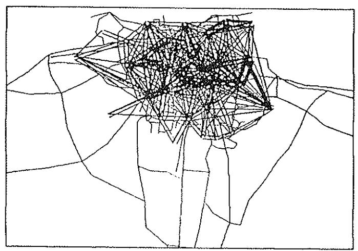
Figure 2.13 Peak hour trip movement pattern from TNPR in 2010
In TNPR the mode split was estimated simultaneously with the trip distribution as mentioned before (equation 2.8). In JMTS, the modal split in the base year was determined on the basis of cordon line surveys. Since there were two different modal split figures observed at the outer and inner cordons, those O-D flows which passed the outer cordon (i.e.Jakarta-Botabek trip) were split in accordance with the corresponding figure of 67 public: 33 private transport whereas for other O-D flows (internal trips not crossing the Jakarta border) the split was 49:51. The overall public transport share was calculated from the two observed modal splits by the formula:
MSpub=(PubShare<sub>out</sub>*Trips<sub>out</sub>+ PubShare<sub>in</sub>*Trips<sub>in</sub>)/ Trips<sub>total</sub> [2.12] where:
PubShare<sub>out</sub> and Trips<sub>out</sub> = Results of outer cordon survey. PubShare<sub>in</sub> and Trips<sub>in</sub> = Results of inner cordon survey.
For the forecast year, JMTS determined the modal split externally (i.e.using certain proportions between particular zones) or using no behavioral model. In comparison of the modal split analysis, the inclusion of motorcycles in the ITSI model is very good, since this mode of transport is quite common in developing countries and thus its inclusion is worthwhile. On the other hand, a limitation of this study was to analyse the change of trips by public modes only, aggregated over
Table 2.2. Predicted modal shares per weekday
| Year | Public Transport | Private | Remarks | |
|---|---|---|---|---|
| Base year | 1990 | 52.5 | 47.5 | % |
| ITSI | 2005 | 50.0 | 50.0 | % |
| TNPR | 2010 | 55.0 | 45.0 | % |
| JMTS | 2015 | 59.0 | 41.0 | % |
Source: compiled from proposal reports
all purposes and for all day. This is inflexible and to some extent is not realistic to consider that the modal split would not change if public transport facilities are improved, whereas in reality such changes are very likely to occur.
The dual-gravity model used in TNPR has the advantage of more detailed results and the inclusion of trip purpose. However, its complexity of analysis requires highly skilled analysts to process. The modal split model used in JMTS was not a behavioral type of model and a drawback of this study is the loss of person type and trip characteristics in the aggregated zonal data.
Looking at the results, the prediction of modal splits in the horizon year between public and private transport in each study can be seen in Table 2.2. This table shows that the predicted public transport share in each study ranged from 50% in 2005 in ITSI to 59% in 2015 in JMTS, bearing in mind that the strategies envisaged were also different. Thus, all these studies forecast a reversal of the historic trends in modal split, against a background of increasing income and car ownership.
2.6.5 Trip assignment
Whereas there were two type of techniques used for assigning private vehicles, for public transport trips the all-or-nothing assignment technique was used in all three studies. The assignment was based on peak hour models. In all three studies the inputs into the model were the transportation network and trip matrices. The network consisted of the road, bus and railway.
In ITSI a capacity-restrained trip assignment procedure was used for road vehicles, including buses. The trip matrices consist-ed of public mode users, cars and motorcycles. The trip matrices were divided by three and assigned to the networks three times respectively. In every step the mode split model divides the public mode trips into bus and railway trips according to travel times and costs of both modes, which were calculated through a minimum path route of each network. The routes were not changed in these assignments for public modes, while the travel times were changed through the increase of road traffic in each assignment step.
In TNPR the trip assignment model adopted was the capacity-restrained model for private trip. Public transport trips were assigned to the public transport network on a mode by mode basis. In JMTS the model used was user equilibrium assignment. In comparing trip assignment for private traffic, the capacity restraint model used in ITSI and TNPR is a slightly less advanced approach compared with the user equilibrium approach used in JMTS. On the other hand, JMTS was simple since just used distance for assigning public transport trip which then took the shortest path between origin and destination. Looking at the public transport networks, there are no significant differences between the studies. All three networks consist of bus-based and rail-based modes. However, the TNPR model seems to be more detailed. For example, it distinguished the waiting times for bus and railbased modes to be 1/2 and 1/4 the headway. whereas in the other studies they were both assumed as 1/2 the headway.
2.7. Discussion of demand modelling methodologies and their results
The type of trip demand models used in all three studies, which were based on the usual 4-stage model, is now under review due to certain weaknesses. They are not fully representing trip behavior or taking into account the effect of network congestion on trip generation, and the development in many areas which affect transportation, such as telecommunication and information technologies like route guidance are not properly represented.
Many alternative models are being developed to improve the basic 4-stage model. for example, by introducing more feedback loops. There are also more radical attempts to understand trip making based on individual or household activities, as in the Disaggregate Travel Demand Model (DTDM). the Household Activities Travel Simulator (HATS) model or base the model on other constraints, as in the travel budget model. On the other hand, there have also been attempts to simplify or modify current models, due to the different characteristics between the developed world, where these types of model originated, and the developing countries (see Dimitriou, 1990 for example). However, the conventional 4-stage models are still adopted in many studies around the world. It appears that this will continue for some years ahead until the new generation of models have been successfully applied, have proved easier to use and give better results.
From the aspects investigated, the significant differences between the results of the three studies are not surprising as this simply reflects the consequences of using the different models and data inputs. This is in line with the finding of Mackinder and Evans (1984), that variation in the external inputs are as important as differences in model specification, accounting for almost 50% of the error produced. Equally, although using the same data input, the different
results demonstrate the effect of the different models used
III. CONCLUSION AND RECOMMEN-DATION
This case study shows that there is still some co-ordination problem faced in infrastructure development in Indonesia as demonstrated by this conflicting plans. Although to co-ordinate all of these studies special agencies exist at all level of government (e.g. the Ministry of National Development Planning Agency at the national level), also these studies have to follow a general guidance in the form of the Area Master Plan made by the City Council. However, the interest of their own institution made the outcomes differ between studies. In addition, the discrepancy in policies among those authorities accentuated the problems of overlapping or even conflicting plans.
From the assessment carried out, it appears that all of the studies have their strengths and weaknesses. However, overall, the JMTS methodologies offered slightly more advantages. Their demand modelling data, which was based on zonal statistical data, is more commonly available and can be updated regularly. Also, despite their rather coarse approach in some respects, their accuracy has proved to be quite good.
Therefore, based on the strengths and weaknesses of the methods used in these studies, a combination of all of them might give even better results. Moreover, they could all improve their methodologies by considering other important issues, as mentioned previously (e.g. the inclusion of motorcycle trips).
IV. REFERENCES
Allport, R.J. and J.M. Thomson. 1990.. Study Of Mass Rapid Transit In Developing Countries. TRRL Contract Report 188, Crowthorne, U.K.
- Buchanan, Colin and partners et al. 1992. Transport Network Planning And Regulation (TNPR) study. Report for the Ministry of Communications, Republic of Indonesia, Jakarta.
- Dimitriou, H.T (ed.) .1990. Transport Planning For Third World Cities. London: Routledge, London
- Dressbach, F. and G. Wessels, G. 1992... Jakarta Mass Transit System Study. Report to the Ministry of Research and Technology, Republic of Indonesia, by Deutsche Gesellschaft für Technische Zusammenarbeit GmbH. Eschborn, Federal Republic of Germany.
- Fouracre, P. R, R.J. Allport and J.M. Thomson. 1990. "The Performance and Impact of Rail Mass Transit in Developing Countries". TRRL Research Report 278, Crowthorne, U.K.
- Halcrow Fox (1996). Blok M Kota Basic Design, Transportation Planning Work Package. Report for The Government of Indonesia, DKI City of Government of Jakarta.
- Inter Departmental Working Group.1993. Jabotabek Urban Mass Transit Preparation Program (Consolidated Network Proposal). Report prepared for the Ministry of Communications, Republic of Indonesia, Jakarta, Indonesia.
- JICA (Japan International Co-operation Agency). 1990. The Study On Integrated Transportation System Improvement (ITSI) By Railway And Feeder Service in Jabotabek Area. Report for the Ministry of Communications, Republic of Indonesia, Jakarta.
- Mackinder and Evans. 1984. The Accuracy of British Transport Studies. TRRL Special Report 699, Crowthorne, U.K.