

I. INTRODUCTION
Travel flow data, e.g. movement of passengers, from origin i to destination j can be estimated using regression models. The regression model can be written as:
\[T_{ij} = \beta_0 + F_{ij}\beta_1 + O_i\beta_2 + O_j\beta_3 + \varepsilon_{ij};\]
\[i = 1, ..., n_2; j = 1, ..., n_2\]
(1)
where \(T_{ij}\) denotes a dependent variable which represents a flow between a given pair of zones i and j. The index i refers to the zones belonging to a set of \(n_i\) zones at the origin and the index j represents one of the \(n_2\) zones at the destination. The same notation is used to model both inter-urban flow data where the originating zones are distinct from the zones at the destination and intra-urban flow data where the set of zones in origin is identical to the set of zones in destination. In that particular case, \(n_i\) would be equal to \(n_2\). One of the earliest examples of this type of modeling in urban context is the model by
Domencich, Kraft, and Valette (1968). A more recent example can be found in Algers (1984), Bowman and Ben-Akiva (2001), Munshi (1993), Jovicic and Hansen (2003). The explanatory variables of this model usually include: (1) Flow or network variables, \(F_{ij}\), which are usually refer to level of service (LOS) variables, for instance travel cost, on-vehicle travel time, out-of-vehicle travel time, fare, frequency, etc; (2) Socio-economic variables (population, income, employment, parking cost, number of cars per household, etc.) associated with the origin, \(O_i\); and (3) Socio-economic variables associated with the destination, \(O_j\). \(\beta_0\) is a constant term and \(\beta_0\), \(\beta_1\), \(\beta_2\) and \(\beta_3\) are coefficients associated with the variables described above.
Because of omission of variables or because of lack of data, the model often cannot capture all relevant factors related to the geographic structure. For instance, a shopping trip to one area may be explained by the absence of other shops with comparable characteristics in neighboring areas. Similarly, if two contiguous destinations have equivalent shopping facilities (shopping malls, for instance), these destinations may be close substitutes for the shoppers of the neighboring zones (Fotheringham and O'Kelly, 1989). The fact of omitting these factors gives rise to some spatial autocorrelation in the regression errors (spatially correlated and/or heteroskedastic), or in another word the error terms do not have the same variance across space. For these reasons, the error term \(\mathcal{E}_{ij}\) in eq. (1) will reflect this situation, and neglecting these error term will lead to bias, and inconsistent in the parameters being estimated (Cliff and Ord, 1981; Anselin and Bera, 1998). To overcome this problem, many solution has been proposed to model the spatial autocorrelation in the dependent variables. An alternative approach is to explain the spatial autocorrelation by adding extra variables to the deterministic part of the model. Using the ideas of in Fotheringham (1983), one could incorporate some intervening regions' variables to capture competing destination effects, competing originating effects and competing network effects. Another possibility is to use the Wills (1986) flexible general gravity-opportunities model which contains both the intervening opportunity model and gravity model as special case. Different from these two approaches, the recent effort proposed by Bolduc et. al. (1992) suggested to handle spatial autocorrelation by incorporating systematic influence on spatial trip correlation by modeling it through the error term. With this approach, we can test whether the intervening region's variables capture the entire spatial correlation structure or just a part of it.
While those approaches may provide alternatives to the solutions, however these approaches are not very instructive on how to improve the model when the assumptions are hurt. To cope with these problems I suggest extending the analytical toolkit by incorporating exploratory spatial data analytical tools (ESDA) into the model evaluation. This tool allows the researcher to monitor the spatial structure of the resulting estimation errors and guide him or her in the process of improving the accuracy of the parameter estimates, and can improve the specification of a given model if there is structure in the error terms. Moreover, this tool can map the statistics of these errors and reveal where the non-stationarity occurs.
The remainder of the paper consists of four sections. I first outline how principles from ESDA are relevant in the analysis of flow data. Specifically, I start by briefly reviewing the concept of ESDA and how it can be applied to spatial data: (1) areal data and then extend that technique to (2) flow data. I next outline some recently developed approaches that focus on "local" indicators of spatial association (or LISA) and discuss how these may be used to detect hot spots and spatial outliers on network and followed by two illustrations: first is a simple illustration of ESDA applied to areal data and the second illustration is an application to flow data. This paper closes with some thoughts on potential extensions and conclusion.
II. EXPLORATORY SPATIAL DATA ANALYSIS
Formally, the presence or absence of pattern is indicated by the concept of spatial autocorrelation, or the co-incidence of similarity in value with similarity in location. In other words, when high values in a place tend to be associated with high values at nearby locations, or low values with low values for the neighbors, positive spatial autocorrelation or spatial clustering is said to occur. In contrast, when high values at a location are surrounded by nearby low values, or vice versa, negative spatial autocorrelation is present in the form of spatial outliers. The point of reference in the analysis of spatial autocorrelation is spatial randomness, or the lack of any structure. For example, under spatial randomness, the particular arrangement of the distribution of the errors of a regression based on travel flow data on a given road network would be just as likely as any other arrangement, and any grouping of high or low values in a particular zone would be totally misleading.
Recently, the set of methods for structuring the visualization of spatial data has been referred to as exploratory spatial data analysis, or ESDA. As defined by Anselin (1994, 1998, 1999a), ESDA is a collection of techniques to describe and visualize spatial distributions; identify atypical locations or spatial outliers; discover patterns of spatial association, clusters, or hot spots; and suggest spatial regimes or other forms of spatial heterogeneity (changing structure or changing association across space). Central to this conceptualization is the notion of spatial autocorrelation or spatial association, i.e. the phenomenon where local similarity (observation in spatial proximity) is matched by value similarity. As such, ESDA forms a subset of exploratory data analysis or EDA (Tukey 1977), but with an explicit focus on the distinguishing characteristics of geographical data, and specifically ESDA techniques formally focus on the detection of global and local patterns of spatial autocorrelation (Anselin, 1995).
In the next section I will introduce the formal definition of Moran's I that is commonly used to detect global pattern and LISA that is commonly used to detect local pattern of spatial autocorrelation. I then extend the concept of LISA to work with flow data.
2.1. Tests for Global Spatial Autocorrelation - Moran's I
Moran's I is the most common measure for assessing spatial autocorrelation. This is the measure that will be used to illustrate the existence of network autocorrelation. Calculation of the index, represented by I, is as follow:
\[I = \frac{\sum_{i=j}^{n} \sum_{i \neq j}^{n} w_{ij} (x_{i} - \overline{x})(x_{j} - \overline{x})}{S^{2} \sum_{i=j}^{n} \sum_{i \neq j}^{n} w_{ij}}\](2)
where \(S^2 = \frac{1}{n} \sum_{i=1}^{n} (x_i - \bar{x})^2\), \(x_i\) denotes the observed value at location \(i, \bar{x}\) is the average of the \(\{x_i\}\) over n locations, \(w_{ij}\) the spatial weight measure defined as 1 if location i is contiguous to location j and 0 otherwise. In the network case: \(x_i\) is the value of variable x on arc or link i; \(\overline{x}\) is the mean of variable x across all arcs; n is the number of arcs; and \(w_{ij}\) is a weight indicating if arc i is connected to arc j (for example, 1) or if it is not (for example, 0).
The expected value and variance of the Moran I for sample size n could be calculated according to the assumed pattern of the spatial data distribution (Cliff and Ord 1981, Goodchild 1986).
For the assumption of a normally distribution,
\[E_n(I) = -\frac{1}{(n-1)},\tag{3}\]
\[VAR_{n}(I) = \frac{n^{2}w_{1} - nw_{2} + 3w_{0}^{2}}{w_{0}^{2}(n^{2} - 1)} - E_{n}^{2}(i),\] (4)
For the assumption of a randomly distribution,
\[E_R(I) = -\frac{1}{(n-1)},\tag{5}\]
\[VAR_{R}(I) = \frac{n((n^{2} - 3n + 3)w_{1} - nw_{2} + 3w_{0}^{2}) - K_{2}((n^{2} - n)w_{1} - 2nw_{2} + 6w_{0}^{2}}{w_{0}^{2}(n^{2} - 1)} - E_{R}^{2}(I)\] (6)
where \[K_2 = \frac{n\sum_{i}^{n} (x_i - \bar{x})^4}{(\sum_{i}^{n} (x_i - \bar{x})^2)^2}\], \(w_0 = \sum_{i}^{n} \sum_{j}^{n} w_{ij}\), \(w_1 = \frac{1}{2} \sum_{i}^{n} \sum_{j}^{n} (w_{ij} + w_{ji})^2\),
\(w_2 = \sum_{i}^{n} (w_i + w_i)^2\), \(w_i\) and \(w_i\) are the sum of row i and column i of the weight matrix respectively.
The test on the null hypothesis that there is no spatial autocorrelation between observed values over the n locations can be conducted based on the standardized statistic as
\[Z = \frac{I - E(I)}{\sqrt{VAR(I)}} \,. \tag{7}\]
A fundamental concept in the analysis of spatial autocorrelation is the spatial weights matrix. This is a square matrix of dimension equal to the number of observations, with each row and column corresponding to an observation. Typically, an element \(w_{ij}\) of the weights matrix W is non-zero if locations i and j are neighbors, and zero otherwise (by convention, the diagonal elements \(w_{ii}\) equal zero). A wide range of criteria may be used to define neighbors, such as binary contiguity (common boundary) or distance bands (locations within a given distance of each other), or even general "social" distance. The spatial weights matrix is used to formalize a notion of locational similarity and is central to every test statistic. In practice, spatial weights are typically derived from the boundary files or coordinate data in a geographic information system (GIS). Figure 1 shows a simple illustration how a 9-by-9 weight matrix is constructed from nine hypothetical zones.
Weight matrices made of ones and zeros are common in autocorrelation analysis. This appears to have had its origin in the use of boundaries and transport linkages to assess contiguity for the weight matrix elements. Areas
shared a boundary or transport link, or they did not. Similarly, in the network case, an arc is connected to another or it is not. It should be apparent that weight matrices may contain higher levels of spatial (or network) ordering than such dichotomous systems. Extensive discussion of the construction of weight matrices for flow data will be given in section 2.3
| Γ Α | A | В | C | a | | l E | | F | Н | 1 r | ||||
|---|---|---|---|---|---|---|---|---|---|---|---|---|
| A | ļ B | C | A | 0 | l | 0 | 1 | 0 | 0 | 0 | \(\frac{\mathbf{n}}{0}\) | 0 |
| В | 1 | 0 | 1 | 0 | 1 | 0 | Ů, | 0 | 10 | |||
| D | Е | F | 0 | 1 | 0 | 0 | 0 | t i | 0 | 0 | 0 | |
| D | 1 | 0 | 0 | 0 | 1 | 0 | Ī | 0 | 0 | |||
| G | Н | T | E | 1 0 | 1 | 0 | I | 0 | 1 | 0 | Ī | 1 0 |
| ٠ ا | 11 | 1 | F | 0 | 0 | 1 | 0 | 1 | 0 | 0 | 0 | |
| 1 | G | 0 | 0 | 0 | 1 | 0 | 0 | 0 | 1 | 0 | ||
| H | 0 | 0 | 0 | 0 | 1 | 0 | 1 | T- | ||||
| 0 | 0 | 0 | 0 | 0 | I | 0 | 1 | 0 | ||||
| (a) | · · · · · · · · · · · · · · · · · · · | (b) | ||||||||||
Figure 1
(a) A hypothetical map of zones, (b) W, the binary contiguity matrix of the map based on rook contiguity criteria, i.e. sharing the common border.
2.2. Tests for Local Spatial Association - LISA
To investigate the spatial variation as well as the spatial associations, some local measurements of spatial statistics can serve such a purpose. In identification of local spatial patterns, there are usually two issues in concern:
- (1). Is the observed value at location i surrounded by a cluster of high or low value?
- (2). Is the observed value at location i surrounded by similar (dissimilar) neighbors?
Local indicators of spatial association (LISA) provide a measure of the extent to which the arrangement of values around a specific location deviates from spatial randomness. This statistic is designed not only to find clusters of high or low values, but also to find hot-spots or outliers (low values surrounded by high values or high values surrounded by low values).
A general framework for LISA is outlined in Anselin (1995), where it is derived from global statistics, the Moran I. Formally, LISA is defined as follow:
\[Ii = Z_i \sum_{j,j \neq i}^n w_{ij} Z_j, \tag{8}\] where the observations Zi and Zj are in standardized form (with mean of zero and variance of one). The spatial weight wij are in row-standardized form. So, Ii is a product of Zi and the average of the observations in the surrounding locations.
The corresponding global Moran I statistic can be obtained by calculating the average of local Morans (Anselin 1995).
\[I = \frac{\sum_{i=j,j\neq i}^{n} \sum_{i}^{n} w_{ij} Z_{i} Z_{j}}{S^{2} \sum_{i=j,j\neq i}^{n} \sum_{i}^{n} w_{ij}} = \frac{1}{n} \sum_{i}^{n} (Z_{i} \sum_{j,j\neq i}^{n} w_{ij} Z_{j}) = \frac{1}{n} \sum_{i}^{n} I_{i}\](9)
with the standardized Zi and row-standardized wij., \(S^2 = \frac{1}{n} \sum_{i=1}^{n} Z_i^2 = 1\) and
\[\sum_{i=j,j\neq i}^{n}\sum_{j,j\neq i}^{n}w_{ij}=n\]
2.3. The LISA Statistics for Flow Data, \(L_{ij}\)
Similar to the \(I_j\) statistic which is defined in the context of lattice data, \(I_i\) in equation (8) can also be generalized to flow data. If in equation (8) we let i denote the flow from i to j, j the flow from k to l, and n the number of flows, it can be directly applied to flow data. Let \(z_{ij}\) denote flows between each pair of zones. Then, given a spatial weight matrix \(W = [w_{ij,kl}]\), we can define a local Moran for flow data as follow:
\[L_{ij} = z_{ij} \sum_{kl \in J_{ij}} w_{ij,kl} z_{kl}\] (10)
Since equation (10) still is Ii statistic, the intuition of the measure is still valid when applied to flow data. Computing this statistic for flow which is associated with an origin-destination pair (i,j) is quite different from lattice data. The difference is mainly due to the way the spatial weight matrix of flow-data defined. In area data the weight matrix may be defined as a contiguity matrix which is based on common boundary, and in point data the weight matrix may be defined as a distance matrix. Similarly we can also apply that concept for flow data where the notion of association between flows are defined as illustrated in Figure 2 as follow:
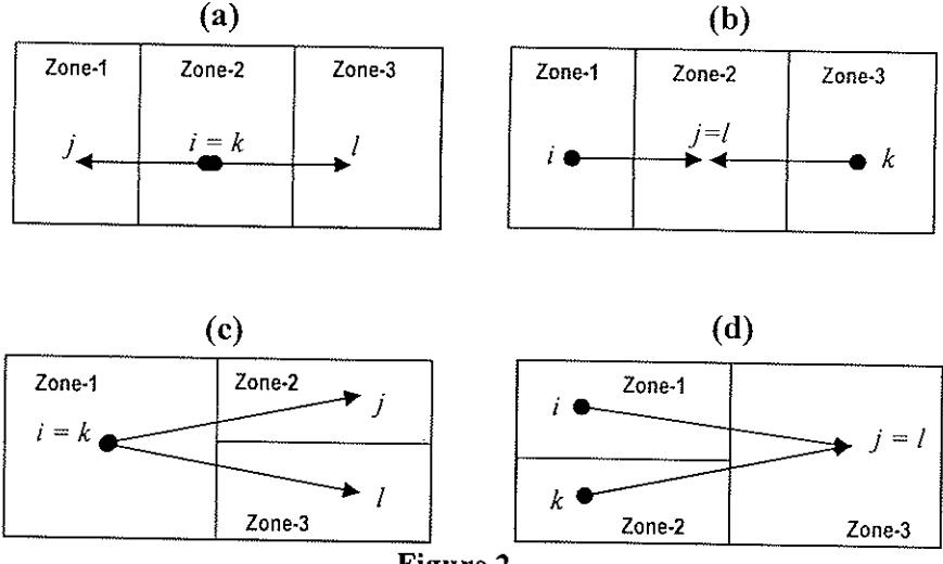
Figure 2. The illustration of spatial association in flow data
- (a) shared only the common point or zone in their origin;
- (b) shared only the common point or zone in their destination;
- (c) not only shared the common point or zone in their origin but also have their destinations being neighbor (contiguity or within a specific distance band);
- (d) not only shared the common point or zone in their destination but also have their origins being neighbor (contiguity or within a specific distance band).
The notion of a weight matrix shown in (a) and (b) is introduced by Black (1992) whose defines a binary spatial weight matrix based on the geographical configuration of the zones, the origins or destinations. Two links are considered to be neighbors (weight equals one) if they are (directly) interconnected. We will consider two different spatial weight matrices of this kind. First, we can let the weight equal one for all flows from a zone i, see Figure 2 (a). With this definition, we can assess whether all flows from i are small or large, independent of destination j (and vice versa).
\[L_{i.}^{*} = \frac{\sum_{j} z_{ij} - n\overline{z}}{s\{[(t-1)n - n^{2}]/(t-2)\}^{1/2}}\](11)
\[L_{,j}^{\bullet} = \frac{\sum_{i} z_{ij} - n\overline{z}}{s\{[(t-1)n - n^2]/(t-2)\}^{1/2}}\](12)
where t is the number of flows, and z is the average and s is the standard deviation of flows between all pairs of origins and destinations, and n equals the number of zones, and z may be approximately equal to zero, for instance if \(z_{ij}\) are residual flows from a properly specified regression model.
The illustrations in Figure 2(c) and 2(d) are provided to represent and capture the notion of intervening opportunities and competing destination model. The notion of spatial association here is an association that falls back on the spatial weight matrix among zones, in other words the configuration of zones. Two binary spatial weight matrices can be defined in this respect as illustrated in Figure 2(c) and 2(b), respectively:
\[W^{d} = [w_{ijkl}] = 1 \text{ if } i=k \text{ and } w_{jl} = 1, \text{ and } 0 \text{ otherwise.}\] (13)
\[W^0 = [w_{ij,kl}] = 1 \text{ if } j = l \text{ and } w_{ik} = 1, \text{ and } 0 \text{ otherwise.}\] (14)
where \(w_{ij}\) denotes elements of the traditional binary spatial weight matrix, i.e. \(w_{ij}\) equals one if i and j are neighbours, and zero otherwise.
Although a binary spatial weight matrix is often used in applications, it is often seen only as a first approximation, and more general forms of weight matrices should be considered. It is often, however, difficult to single out one particular weight matrix from a number of candidates. I have also employed a more general form, with parameterized spatial weights,
\[W^{\Box} = [w_{ij,kl}] = (d_{il} + d_{jk})^{\delta}\] (15)
where \(\delta\) is the parameter, and \(d_{ij}\) denotes the distance between zone i and j.
2.4. Generalized Forms for LISA statistics
According to Getis and Ord (1992), Ord and Getis (1994) and Anselin (1995), it is assumed that observed values are randomly distributed over space under the hypothesis of no spatial association. Each attribute value (xi) is in equal probability at every spatial unit over the space (p(xi)=1/n). However, in many studies, the spatial unit is not always defined regularly in a spatial sense. It is then questionable that the probability of the sampled value is inversely proportional to the number of spatial units. One example is the Census tract that is defined to include about 4,000 people. Thus, tract area varies greatly between urban and rural tracts. In the pattern of population distributed over space, it is more reasonable to assume that the probability of the population density observed at location i is proportional to its areal share of the space \((p(xi) = ai/\Sigma jaj)\). In this case, local Moran defined above will not hold. The traditional permutation test will be inappropriate if each observation is sampled in equal probability.
The generalized form for LISA can be defined as
\[I_i^* = Z_i \sum_{j,j \neq i}^n g_{ij} Z_j \tag{16}\] where \(\{Zi\}\) is a series of standardized observations, \(\{g_{ij}\}\) is a generalized row standardized spatial weight matrix \((g_{ij} = w_{ij}p_j / \sum_{i=1}^{n} w_{ij}p_j)\).
The expected values and variances of the generalized LISA can be defined as follow:
\[E(I_i^*(g)) = \sum_{j,j\neq i}^n g_{ij} E(Z_i Z_j) = Z_i D_{i1} U_{i1}\] (16)
\[Var(I_i^*) = Z_i^2 [D_{i2}U_{i2} + (D_{i1}^2 - D_{i2})U_{i3}] - E(I_i^*)^2\] where pi is the conditional probability (P(V-reflY-text))
where \(p_i\) is the conditional probability \((P(X=x_i|X\neq x_i))\),
\[G_{i1} = \sum_{j,j\neq i}^{n} g_{ij} = 1; \ G_{i2} = \sum_{j,j\neq i}^{n} g_{ij}^{2}; b_{j} = \frac{p_{j}}{1 - p_{j}}; \ U_{i1} = \sum_{j,j\neq i}^{n} p_{j} Z_{j};\]
\[U_{i2} = \sum_{i,j\neq i}^{n} p_{j} Z_{j}^{2}\]; and
\[U_{i3} = \sum_{j,j\neq i}^{n} p_{j} Z_{j} \sum_{j,j\neq i}^{n} b_{j} Z_{j} - \sum_{j,j\neq i}^{n} p_{j} b_{j} Z_{j}^{2}\]
The generalized LISA is equal to its standard forms when each conditional probability \((P(X = xj | X \neq xi), j = 1...n)\) is identical (i.e., p1 = p2 = ... = pn). Compared with the LISA, the generalized forms can reflect the actual spatial distribution without distortion by incorporating the conditional probability into the measurements. The estimated expected values and variances are consistent and the tests are more reliable in spatial problems with a heterogeneous sample distribution (Bao and Henry 1996). With the special case of flow data, zone weights (e.g. population, incomé level, etc) can be employed since the probability of a random variable observed at a specific flow is proportional to its characteristic measurement of its origin or destination. The conditional probability can then be represented by \(p_j = (P(X | P(X | P(X | P(X | P(X | P(X | P(X | P(X | P(X | P(X | P(X | P(X | P(X | P(X | P(X | P(X | P(X | P(X | P(X | P(X | P(X | P(X | P(X | P(X | P(X | P(X | P(X | P(X | P(X | P(X | P(X | P(X | P(X | P(X | P(X | P(X | P(X | P(X | P(X | P(X | P(X | P(X | P(X | P(X | P(X | P(X | P(X | P(X | P(X | P(X | P(X | P(X | P(X | P(X | P(X | P(X | P(X | P(X | P(X | P(X | P(X | P(X | P(X | P(X | P(X | P(X | P(X | P(X | P(X | P(X | P(X | P(X | P(X | P(X | P(X | P(X | P(X | P(X | P(X | P(X | P(X | P(X | P(X | P(X | P(X | P(X | P(X | P(X | P(X | P(X | P(X | P(X | P(X | P(X | P(X | P(X | P(X | P(X | P(X | P(X | P(X | P(X | P(X | P(X | P(X | P(X | P(X | P(X | P(X | P(X | P(X | P(X | P(X | P(X | P(X | P(X | P(X | P(X | P(X | P(X | P(X | P(X | P(X | P(X | P(X | P(X | P(X | P(X | P(X | P(X | P(X | P(X | P(X | P(X | P(X | P(X | P(X | P(X | P(X | P(X | P(X | P(X | P(X | P(X | P(X | P(X | P(X | P(X | P(X | P(X | P(X | P(X | P(X | P(X | P(X | P(X | P(X | P(X | P(X | P(X | P(X | P(X | P(X | P(X | P(X | P(X | P(X | P(X | P(X | P(X | P(X | P(X | P(X | P(X | P(X | P(X | P(X | P(X | P(X | P(X | P(X | P(X | P(X | P(X | P(X | P(X | P(X | P(X | P(X | P(X | P(X | P(X | P(X | P(X | P(X | P(X | P(X | P(X | P(X | P(X | P(X | P(X | P(X | P(X | P(X | P(X | P(X | P(X | P(X | P(X | P(X | P(X | P(X | P(X | P(X | P(X | P(X | P(X | P(X | P(X | P(X | P(X | P(X | P(X | P(X | P(X | P(X | P(X | P(X | P(X | P(X | P(X | P(X | P(X | P(X | P(X | P(X | P(X | P(X | P(X | P(X | P(X | P(X | P(X | P(X | P(X | P(X | P(X | P(X | P(X | P(X | P(X | P(X | P(X | P(X | P(X | P(X | P(X | P(X | P(X | P(X | P(X | P(X | P(X | P(X | P(X | P(X | P(X | P(X | P(X | P(X | P(X | P(X | P(X | P(X | P(X | P(X | P(X | P(X | P(X | P(X | P(X | P(X | P(X | P(X | P(X | P(X | P(X | P(X | P(X | P(X | P(X | P(X | P(X | P(X | P(X | P(X | P(X | P(X | P(X | P(X | P(X | P(X | P(X | P(X | P(X | P(X | P(X | P(X | P(X | P(X | P(X | P(X | P(X | P(X | P(X | P(X | P(X | P(X | P(X | P(X | P(X | P(X | P(X | P(X | P(X | P(X | P(X | P\)
\[=xj|X\neq xi)=a_j/\sum_{i,i\neq j}^n a_i.\]
2.5. Moran Scatterplot
The degree of spatial autocorrelation in a dataset can be readily visualized by means of a special scatterplot, termed Moran scatterplot in Anselin (1995. 1996). The Moran scatterplot is centered on the mean and shows the value of a variable (z) on the horizontal axis against its spatial lag (\(W_z\), or \(\Sigma_i w_{ii} z_i\), i.e., a weighted average of the neighboring values) on the vertical axis. The four quadrants in the scatterplot correspond to locations where high values are surrounded by high values in the upper right (an above mean z with an above mean Wz), or low values are surrounded by low values in the lower left, both indicating positive spatial autocorrelation. The two other quadrants correspond with negative spatial autocorrelation, or high values surrounded by low values (high z. low Wz) and low values surrounded by high values (low z. high Wz). The slope of the linear regression line through the Moran scatterplot is Moran's I coefficient. Moreover, a map showing the locations that correspond to the four quadrants provides a summary view of the overall patterns in the data. Hence, this device provides an intuitive means to visualize the degree of spatial autocorrelation, not only in a traditional crosssectional setting but also across variables and over time.
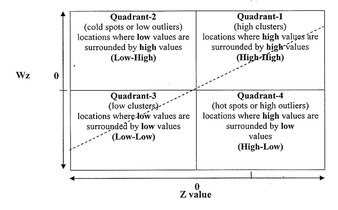
Figure 3. The Layout of Moran Scatterplot, the dash line represents the slope of the linear regression line (Wz on Z), and its slope is the Moran I coefficient.
III. ILLUSTRATION
In this illustration, GeoDa, a simple and user-friendly ESDA software package developed by Anselin and Syabri (2003), is used to conduct exploratory spatial data analysis for areal data and flow data. The purpose of demonstrating the areal data here is to illustrate the basic concepts ESDA before departing to the ESDA techniques for flow data.
3.1. Illustration of the use of ESDA for Areal Data
For purposes here I will use data on the spatial distribution of household consumption in the greater Jakarta metropolitan area of Indonesia. This region is referred to as the Jabotabek metropolitan area, and it comprises 129 subdistricts, covering, in addition to Jakarta, the urban areas of Bogor, Tangerang and Bekasi. This metropolitan region is characterized by internal restructuring, both physical as well as in terms of socio-economic characteristics. The primary pattern is one of decentralization of manufacturing (away from the city center) and concentration of finance and services, changing the nature of urban areas in the core". We consider the spatial distribution of median household consumption in the region, as well as its relation to disposable (household) income in a simple linear consumption function. In Figure 4, the central graph shows a quartile map for household consumption, with the "outliers" highlighted in the center. The districts in question happen to all be near the core of Jakarta, suggesting the existence of a "cluster." While these are the locations that match the outlying data points on the traditional box plot on the right, the latter does not shed light on any "spatial" pattern as in the box map. On the left, a scatterplot with a linear smoother illustrates the slope of the consumption function and how this is affected when the outlying observations are removed from the analysis (the slope of 0.74 on the upper right hand side of the graph is the value obtained without the outliers). Clearly, the selection in one of the graphs is linked to the matching observations on the other graphs.
We further investigate the spatial pattern of consumption expenditures by focusing on the districts with a significant Local Moran and the type of spatial autocorrelation suggested, as illustrated in Figure 5. The graph on the lower right presents the Moran scatterplot and suggest a (significant) degree of positive spatial autocorrelation (Moran's I is 0.54). The local autocorrelation provides a more fine grained view of the association however. The significant districts are shown in the lower left map, with the classification by type of association given in the LISA map at the upper left. Both maps have been zoomed in to provide a better view of the pattern near the core city. While the evidence overwhelmingly suggests a significant "cluster" of high household consumption near the center-city, there is one district that does not fit the mold. In the very center, the Tanah Abang district (identified in the Table on the upper right) shows a significant pattern of negative association, i.e., a low value surrounded by high values. A look at the matching point in the Moran scatterplot confirms that this is indeed a location with below average consumption, surrounded by above average neighbors. This pattern is such that it is highly unlikely to occur under spatial randomness. The district in question is indeed a remaining area of urban decay, where the conversion to business activity, characteristic of the other core districts, has not (yet) taken place.
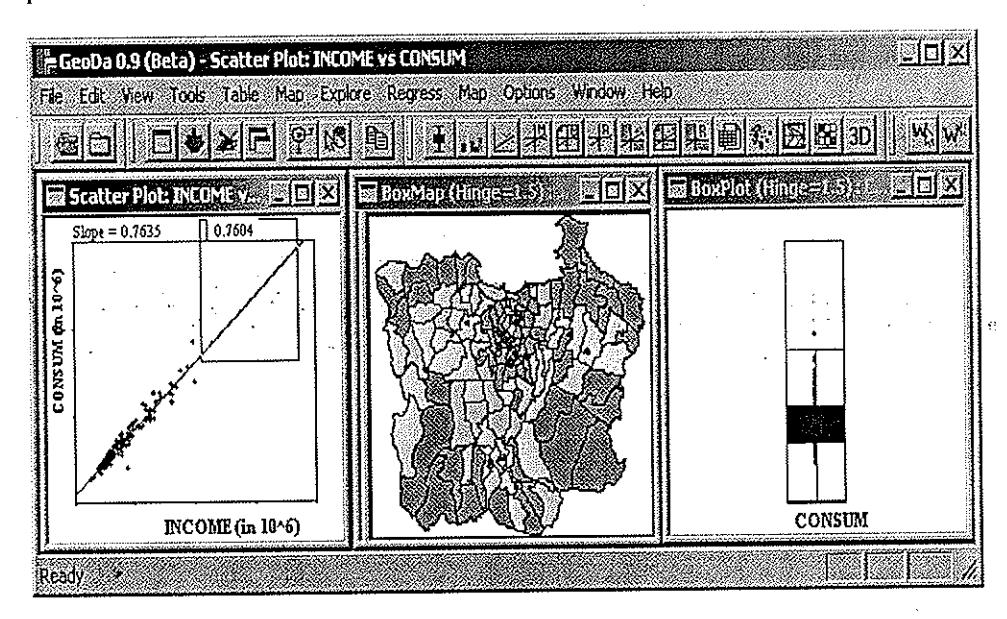
Figure 4 Distribution of household consumption in the Jabotabek region.
As a final illustration, I consider evidence of spatial heterogeneity, or the significant difference between moments of a distribution and model parameters by regional "regimes." In Figure 6, a brush is centered on the core urban area, selecting those districts in the map and in the matching box plot. This also eliminates the selected points from the computation of Moran's I and the slope of the consumption function. The latter, shown in the bottom right graph, is substantially higher than for the data set as a whole (0.90 vs. 0.76), confirming the well-known phenomenon that the propensity to consume (the slope of the regression line) is not constant, but inversely related to income (lower income groups, outside the core districts, have higher propensity to consume). Moving the brush over the map would allow the analyst to interactively assess the degree of change in this parameter over
subregions of the data, suggesting candidate "spatial regimes" for further analysis by means of spatial econometric software.
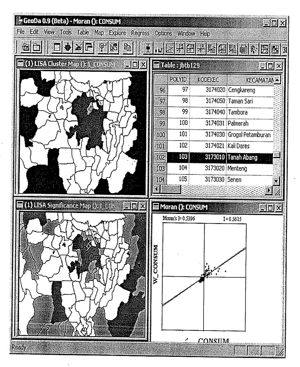
Figure 5 Visualizing local and global spatial autocorrelation for areal data.
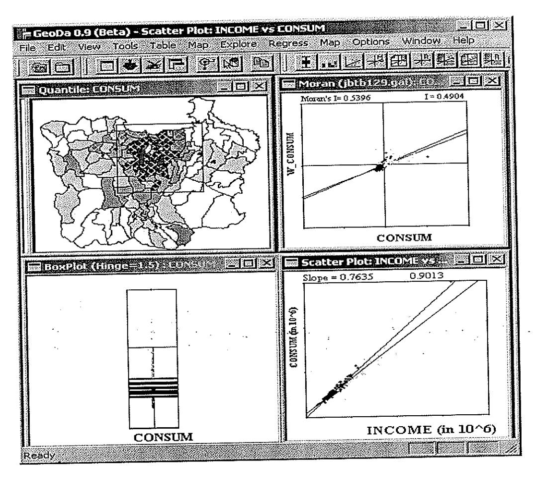
Figure 6 Visualizing spatial heterogeneity.
A "static" description such as the one given here rarely gives proper credit to the type of additional insight generated through a dynamic interaction with the data, especially when complemented with substantive knowledge of the issue at hand (Syabri and Anselin, 2003). Such interaction often provides significant added value over a more traditional data analysis, motivating further work on extending and refining the current framework<sup>iii</sup>.
3.2. Illustration of the Use of ESDA for Flow Data
In this illustration I compute the proposed measures to analyze spatial association of migration flows. The migration model used to generate residuals is a log linear gravity model estimating migration flows between 1965 and 1970 of the major census regions of the United States<sup>iv</sup>. The relative
unemployment in origin zone, the total population in both origin and destination zones, ratio between housing prices in origin and destination zones are used as determinants associated with the origin and destination zones. The distance between zones is used as a determinant describing the friction. There error terms are as usual are assumed to have expectation zero, same variance, and to be independent. Hence, under the null hypothesis of no spatial association we assume that the residuals are not correlated.
There are 9 (nine) zones, and consequently 72 flows and a 72-by-72 arc weight matrix for the network autocorrelation analysis. Clearly for larger zones, we going to run the risk of producing rather cluttered maps if we endeavor to display all flows (for n zones, the number of flows will be \(n^2 - n\)). Figure 7 shows a query for simply showing flows that in and out of the Pacific region with yellow lines represent flows from and to the Pacific region. The dots are simply the centroids of the regions and the lines are symbolized the flows where the width of the line is proportional to the volume of the flow.
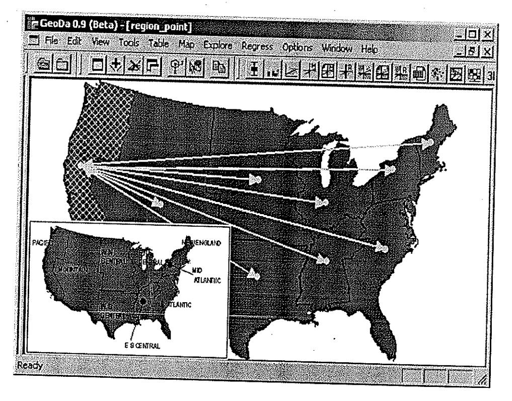
Figure 7. The nine major census regions of the United States.
The map in Figure 8 illustrates the spatial distribution of high values of the residuals that associated with the quadrant-1 of the Moran scatterplot on the left. The spatial association in the residuals is visualized by the Moran scatterplot map, which symbolizes the four quadrants of the Moran scatterplot and suggests a (significant) degree of positive spatial autocorrelation (Moran's I is 0.31).
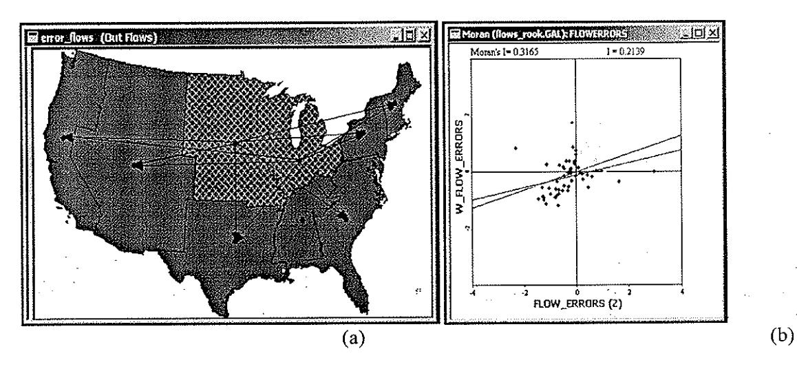
Figure 8. Visualizing the clusters of high values of the residuals.
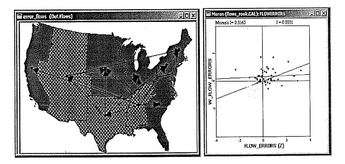
Figure 9. Visualizing the clusters of low values of the residuals.
Fourteen out of sixteen residual flows coming out from W-N Central and E-N Central regions to other regions are among the highest values of residuals (above average residuals) that are surrounded by high-residual flows which suggest a significant cluster. Excluding these clusters out from the analysis changes the Moran I from 0.36 to 0.21 (showed on the top right of the Moran scatterplot with brown color). On the other hand, in Figure 9, the outlying data points of quadrant-3 (locations where low values are surrounded by low values) surprisingly create clusters in the Mountain, W-S Central, and S Atlantic, and East South Central and excluding these clusters out from the analysis changes the Moran I very significantly from 0.36 to 0.03.
As a final illustration, I consider evidence of spatial heterogeneity, or the significant difference between moments of a distribution and parameter of spatial association. In Figure 9, a selection brush is set on the south of area, selecting those regions (Mountain, W-S Central, and S Atlantic, and East South Central) in the map and in the matching Moran scatterplot. This also eliminates the selected points from the computation of Moran's I and changes the slope of the residuals (FLOW_ERRORS vs W_FLOW_ERRORS). The latter, shown in the right graph, is substantially lower than for the residuals as a whole (0.31 vs. 0.03), confirming that the error term (the slope of the regression line) is not constant. Moving the brush over the map would allow the analyst to interactively assess the degree of change in this parameter over subregions of the data, suggesting candidate "spatial regimes" for further analysis by means of spatial econometric software.
These impressive findings indicate a significant level of dependence in the residuals, that is, the error terms cannot be assumed to be spatially independent, and interpret to signal model misspecification. When this error dependence is ignored, the resulting estimator remains unbiased, although it is no longer most efficient. Moreover, the estimates for the coefficient standard errors will be biased, and, consequently, t-tests and measures of fit will be misleading.
Although it is not the purpose of this paper to discuss the remedy of the model, remedial action may involve re-specifying the model. The most commonly used models are based on spatial processes, such as a spatial autoregressive (SAR) or spatial moving average (SMA) process, in parallel to the time series convention. The particular form for the process yields a non-diagonal covariance structure for the errors, with the value and sign of the off-diagonal elements corresponding to the "spatial correlation" (that is, the correlation between the error terms at two different locations).
IV. CONCLUSION AND POTENTIAL EXTENSION
The purpose of this paper is to introduce ESDA as a new tool for exploring flow data by generalizing the global and local statistics of spatial autocorrelation to allow for applications with flow data, and to demonstrate its usefulness in two applications. The application of ESDA to flow data introduces new aspects which merit further consideration on its own. We have explored non-stationarities and identified underlying geographical patterns. The localized statistics as implemented in this paper makes it possible to address how relationships between variables vary over space. We believe that the used measures have improved our understanding of the strengths and weaknesses of the estimated models in terms of a spatial analysis. This understanding can be incorporated into improved and more comprehensive models.
Most current techniques of exploratory data analysis work fine for small to medium-sized datasets. However, increasingly large spatial datasets (with 100,000 to millions observations) become the subject of investigation in spatial data analysis, primarily in application of spatial interaction models where the size of flows become quadratic \((n^2 - n)\). Simple extrapolation of ESDA methods to large datasets is therefore not feasible.
V. REFERENCES
- Anselin, L. and I. Syabri. 2003. GeoDa 0.9 User's Guide. Urbana-Champaign, IL: Spatial Analysis Laboratory (SAL). Department of Agricultural and Consumer Economics, University of Illinois, Urbana-Champaign, IL.
- Anselin, L. 1999a. Interactive techniques and exploratory spatial data analysis. In Geographical Information Systems. 2d ed, ed. P. Longley, M. Goodchild, D. Maguire, and D. Rhind. New York: John Wiley & Sons.
- Anselin, L. 1999b. Spatial econometrics. In Companion in Theoretical Econometrics, ed. B. Baltagi. Oxford: Basil Blackwell.
- Anselin, L. 1998. Exploratory spatial data analysis in a geocomputational environment. In Geocomputation, a primer, eds. P. Longley, S. Brooks, R. McDonnell, and B. Macmillan. New York: John Wiley & Sons.
- Anselin L. and A. Bera. 1998. Spatial dependence in linear regression models with an introduction to spatial econometrics. In Handbook of Applied Economic Statistics, pp.237-289 eds. Amman Ullah and David Giles. New York: Marcel Dekker.
- Anselin, L. 1996. The Moran scatterplot as an ESDA tool to assess local instability in spatial association. In Spatial analytical perspectives on GIS, eds. M. Fischer, H. Scholten, and D. Unwin. London: Taylor and Francis.
- Anselin, L. 1995. Local Indicators of Spatial Association LISA. Geographical Analysis, 27(2), 93-115.
- Anselin, L. 1994. Exploratory spatial data analysis and geographic information systems. In New Tools for Spatial Analysis, ed.M. Painho. Luxembourg: Eurostat.
- Black, W. R. 1992. Network autocorrelation in transport network and flow Systems. Geographical Analysis, 24(3), 207-222.
- Bolduc, D. 1992. Spatial autoregressive error components in travel flow models. Regional Science and Urban Economics, 22(3), 371-385.
- Bowman, J. L. and M. E. Ben-Akiva. 2001. Activity-based disaggregate travel demand model system with activity schedules. Transportation Research Part A: Policy and Practice, Volume 35, Issue 1, Pages 1-28.
- Cliff, A.D., and J. K. Ord. 1981. Spatial Processes, Models, and Applications. London: Pion.
- Fotheringham, A. S. 1983. A New Set of Spatial-Interaction Models: The Theory of Competing Destinations. Environment and Planning A 15: 15-36.
- Fotheringam A. S. and M. E. O'Kelly. 1989. Spatial Interaction Models: Formulations and Applications. Dordrecht: Kluwer.
- Getis, A. and J. K. Ord. 1992. The analysis of spatial association by use of distance statistics. Geographical Analysis, 24(3), 189-206.
- Jovicic G., and C. O. Hansen. 2003. A passenger travel demand model for Copenhagen. Transportation Research Part A: Policy and Practice, Volume 37, Issue 4, pp. 333-349.
- Messner, S., L. Anselin, R. Baller, D. Hawkins, G. Deane, and S. Tolnay. 1999. The spatial patterning of county homicide rates: An application of exploratory spatial data analysis. Journal of Quantitative Criminology 15 (4): 423–450.
- Munshi, K. 1993. Urban passenger travel demand estimation: A household activity approach. Transportation Research Part A: Policy and Practice, Volume 27, Issue 6, pp. 423-432.
- Ord, J.K. and A. Getis. 1995. Local spatial autocorrelation statistics: Distributional issues and an application. Geographical Analysis, 27(4), 286-305.
- Tukey, John W. 1977. Exploratory Data Analysis. Reading, Massachusetts: Addison-Wesley.
- Syabri, I. and L. Anselin. 2001. Visualizing Spatial Autocorrelation with Dynamically Linked Windows. Computing Science and Statistics 33.
- Syabri, I., L. Anselin, and O. Smirnov. 2002. Visualizing multivariate spatial correlation with dynamically linked windows. In New Tools for Spatial Data Analysis: Proceedings of the Specialist Meeting, eds. L. Anselin and S. Rey. Santa Barbara: Center for Spatially Integrated Social Science (CSISS), University of California, Santa Barbara.
<sup>1</sup> The data are from the 1999 Indonesian socio-economic survey, or SUSENAS (BPS 1999).
For an extensive discussion of the substantive issues involved, see, e.g., Firman (1998).
For a recent example of an instance where the use of ESDA through dynamically linked windows generated "surprising" new insights, see Messner et.al. (1999).
The migration data used here has been used in the studies by Tobler (1983), William and Fotheringham (1984), Bexter (1987), and Black (1992).