
Introduction
In modern metropolitan cities, public transportation plays an important role in improving urban environments and reducing traffic energy consumption. An example of this is high-capacity urban rail, which is mainly constructed underground so traffic congestion is not aggravated and air pollution emissions are reduced compared with other means of transportation. Therefore, cities worldwide have built substantial urban rail systems with numerous lines and stations. For example, London has eleven routes with a total length of 402 km, and Tokyo has thirteen routes with a total length of 304 km of urban rail infrastructure. When infrastructure construction for urban rail reaches its limit, it is difficult to create new lines and stations. Therefore, it is important to increase the utilization efficiency and quality of transportation within the existing infrastructure.
Research into urban planning has focused on increasing the number of urban rail users. Transitoriented development (TOD) in particular has become an important paradigm since the early 2000s. TOD is the concept of increasing the number of station users by increasing the density and diversity of land use around the catchment area of urban rail stations and designing roads with easy access to the stations (Cervero et al., 2002). A number of empirical studies have been conducted to determine the impact of land-use density and diversity on the number of station users (Cervero, 1996; Cervero and Kockelman, 1997; Ewing and Cervero, 2001; Cervero and Murakami, 2009; Lin and Shin 2008; Sung et al. 2014; Yoo, 2013). These studies revealed that the land-use density of the station catchment area increases the transit utilization rate. The effect of diversity of land use on the public transportation utilization rate differed in each study. The station's topology is another important factor that may affect the number of passengers. It has been found that stations in the same city perform different functions depending on whether they have a central or a suburban location.
Prior research into topology differences between stations has taken several approaches. Some studies have analyzed the topology of each station using dummy variables for the downtown area and the outskirts of the city (Lee et al., 2013; Lyu et al., 2016). Other studies (Nasri and Zhang, 2014; Arrington and Cervero, 2008) used the distance between the station and the central business district (CBD) and the number of urban railway lines passing through each station (Sohn and Shim, 2010; Jun et al., 2015). However, these methods are limited in their ability to calculate the spatial network centrality of each station, as even if the stations are located in the city center or have the same number of urban railway lines passing through them, they may have different spatial network centralities. Additionally, the distance from the CBD cannot be used as network centrality if the city has an atypical shape. Therefore, a method for calculating the spatial topology of each station based on its status in the urban railway network is necessary.
We used social network analysis (SNA) to examine the relationship between objects through sociograms consisting of nodes and lines. The structure of the network in a sociogram is quantified by centrality indicators, which denote the degree of closeness and connectivity between each object. Various studies have been conducted on the centrality indicator methodology (Han, 2010), and centrality indicators have been applied in urban studies, such as geographical analysis and transportation planning (Porta et al., 2009; Wang et al., 2011; Kang, 2015). However, no studies used centrality indicators for urban railways developed with SNA to analyze the number of passengers and the average distance traveled.
The number of passengers means the total number of passengers getting on and off at each station. The average distance is the average of the distance traveled by passengers boarding at each station. The average distance is obtained by calculating the total travel distance of the people who boarded at each station and dividing this by the number of passengers at each station.
This study aimed to calculate the network centralities of urban railway stations in Seoul using SNA and analyze the effect of this value on the number of passengers and average travel distance from each station. The case study applied SNA centrality indicators to Seoul Metropolitan railway stations. We estimated a regression analysis model with the characteristics of building use in the station catchment areas as the control variables. Furthermore, we compared this methodology to methods of obtaining topology values used in previous studies.
This study is different from previous studies in that it analyzed the factors affecting the average travel distance of passengers. The average travel distance of passengers is related to the service quality of public transportation. Existing studies (MVA Consultancy, 2008; Kato, 2014) have revealed that reducing the travel distance of passengers can alleviate congestion in train coaches and improve the quality of transportation services. Therefore, we included in the analysis the effect of network accessibility on the travel distance of passengers. Thus, this study analyzed not only the effect of network accessibility on increasing the amount of urban railroad usage but also the degree of impact on service quality.
Literature Review
We reviewed previous studies from three perspectives. First, we reviewed prior research on land use in the catchment areas of urban rail stations, which has been shown to have the greatest impact on the number of users at urban railroad stations. Both density and diversity of land use in station catchment areas have been considered important variables for predicting the number of station users in prior TOD research. These studies have identified variables that must be controlled for in this analysis. Second, we reviewed research into the spatial topology of urban railway stations, identifying a variety of methods for analyzing the spatial topology of urban railway stations. Noting these methods' limitations, we demonstrate how the methodology of this study contributes to the literature. Finally, we review a prior urban planning study that used SNA.
Prior Research on Land Use in the Catchment Area of Urban Rail Stations
TOD consists of high land-use density, diverse land use, and a pedestrian-friendly design. Empirical studies on the effects of TOD have focused on how it shapes public transportation usage rates and non-motorized travel. Calthorpe introduced the concept of TOD in the late 1980s and developed its guidelines (Calthorpe, 1993). Cervero and Kockelman (1997) named the components of TOD the three Ds: density, diversity, and design. Analyzing land use and the effect of these indicators on travel patterns, they found that higher density and more diverse land use decreased car traffic. Additionally, public transportation increased when the city's design elements were more pedestrian-friendly. Ewing and Cervero (2001) summarized a number of TOD studies and found that the socioeconomic characteristics of passengers as well as density, diversity, design, and local access, influenced travel demand. They added destination accessibility as a fourth element of TOD, creating the four Ds. Ewing et al. (2007) extended the concept from four Ds to five Ds, adding distance-to-transit (Ewing et al., 2007). Several studies (Li, 2012; Dirgahayani and Choerunnisa, 2018) have analyzed and evaluated TOD based on the five Ds. As an increasingly advocated concept supported by substantial empirical evidence from American
cities, TOD has become one of the key planning methods for managing urban growth intelligently in the twenty-first century (Ewing et al., 2007; Hamin and Gurran, 2009).
TOD studies in Asian cities have been conducted since the early 2000s. TOD planning concepts have been applied in Asian cities experiencing suburbanization and traffic congestion, particularly in China. In a Hong Kong case study, Cervero and Murakami (Cervero and Murakami, 2009) concluded that TOD is more effective in increasing transit ridership than transit-adjacent development. In Taipei, Lin and Shin (2008) found that TOD planning increases ridership when the built environment is consistent with TOD principles. However, the impact of TOD, particularly the effect of diversity, may differ between American and Chinese cities because of cultural differences (Lin and Shin, 2008). One such example is provided by Zhang (2004) in a study that demonstrated that mixed land-use development near a transit center does not significantly impact transit mode choices. This analysis was not limited to Hong Kong. Sung et al. (2014) and Yoo (2013) discovered that mixed land use was a factor in lowering the demand for public transportation in Korea, contrary to its role in major US cities. Thus, it is necessary to identify the impacts of TOD planning concepts on transit mode choices and transit ridership in specific national contexts.
Analysis of the effects of TOD factors on public transportation utilization reveals that the landuse density of the station catchment area is a factor that increases the transit utilization rate, although there are differences among cities. On the other hand, the effect of diversity of land use on the public transportation utilization rate differed in each study. It was found to be a positive factor for the use of public transportation in North America. However, research has shown that diversity of land use negatively affects public transportation usage or has a negligible effect in Asia.
Spatial Topology of Urban Railway Stations
Several limitations have been identified in empirical studies that analyzed the relationship between TOD and public transport use. One of these is that station topology was not considered; existing studies have compared stations on the same basis, ignoring the functional characteristics arising from the area where the subway station is located. Therefore, these studies were not able to make objective judgements on the impact of land-use characteristics on public transport users. Further studies have been conducted to overcome this limitation, which can be divided into three types.
First, there are studies that classified stations into several clusters based on their locations and characteristics and analyze the features associated with TOD for each cluster. Lee et al. (2013) classified subway stations based on the regional functions given in the urban planning using two clusters: one with three options (CBD, sub-central area, and fringe area) and one with four options (CBD, inner suburbs, outer suburbs, and periphery areas). For each cluster, they analyzed the relationship between TOD land use and ridership. The results indicated that subway riders from stations in CBD locations and from fringe or peripheral areas were most influenced by density, whereas riders from stations located in sub-central areas or inner and outer suburbs were most influenced by diversity of land use. Lyu et al. (2016) calculated the 'transit', 'development', and 'oriented' indicators for urban rail stations located in the analysis area. They classified each station into six clusters based on the index. They analyzed the catchment area of each station for each cluster, revealing a difference in the indicators associated with TOD in each cluster. This method partially reflects the differences in the stations' topologies, but the classification criteria for the clusters were ambiguous. Additionally, differences within the same clusters were not examined.
Second, there are studies that measured the topology of stations using the distance from the CBD to each subway station. Nasri and Zhang (2014) analyzed the effects of land-use characteristics of the catchment areas of stations on vehicle miles traveled (VMT) in Washington D.C. and Baltimore. The results of this study indicated that people living in TOD areas tended to drive less, reducing their VMT by around 38% in Washington, D.C. and by 21% in Baltimore compared to the residents of non-TOD areas, including areas with similar land-use patterns. They controlled for the topology of each station by including a variable measuring the distance from the CBD to analyze the effect of land use in the catchment areas on transit patterns. Arrington and Cervero (2008) analyzed seventeen TOD projects of varying sizes in four urban areas and found that people living in TOD areas used transit two to five times more often for commuting trips compared to those living in non-TOD areas. This study also measured the topology of each catchment area using the CBD distance along with the land-use density of each area. These studies (Nasri and Zhang, 2014; Arrington and Cervero, 2008) assumed that the distance between the CBD and each station affected the traffic patterns of passengers who used a station. In addition, the results showed that the longer the distance from the CBD, the greater the amount of traffic and the distance of the average ride. However, taking one point (the CBD) as reference point for the topology does not capture the variety of land uses that are prevalent throughout the city.
Third, a number of scholars have used the possibility of transfer or the number of subway lines passing through to measure the topology of a station. Kuby et al. (2004), Zhao et al. (2013) and Sung et al. (2014) estimated regression models of rail use in the United States, China, and Korea, respectively. These studies used dummy variables indicating whether transfer was possible to capture the topology of each station. In contrast, Sohn and Shim (2010) and Jun et al. (2015) used the number of lines passing through each station, a continuous variable, to capture station topology. Despite differences in how the variables were measured, the above studies have shown that the number of passengers increases if transfer is possible at a station or if many lines traverse the station. However, this approach does not account for the geographical location of a station in the city, and it cannot consider a station's relationship with other stations connected through the urban railway network.
As discussed above, many studies have analyzed how the topology of stations affects ridership. Nevertheless, there are limitations in the way that topology has been operationalized. SNA is a new method that overcomes these limitations and quantifies the relationship among objects in a network. SNA concepts are theoretically grounded in the insights provided by Simmel (1950) and Durkheim (1984) and are methodologically grounded in classical graph theory (Moody and White, 2003). SNA treats social relationships as networks consisting of nodes and links (also called edges, ties, or connections). The nodes represent the individual actors within the network, and the links indicate the relationships between the actors. Research in a number of academic fields has shown that social networks are identifiable in many types of organizations—from families to nations—and they play a critical role in determining the way in which problems are solved, organizations are run, and the degree to which individuals succeed in achieving their goals (Passmore, 2011). SNA has been used in the social sciences and, increasingly, in the physical sciences.
Prior Urban Planning Studies Used SNA
Most studies using SNA in urban planning considered the relationship between network centrality and urban spatial structure. Porta et al. (2009) applied SNA to road networks to calculate the centroid index of a city and compared it with commercial distribution. They reported that streets where the centrality index was high had more retail outlets. Also using road networks to calculate
urban centrality indices, Wang et al. (2011) analyzed the influence of centrality on population and worker density, while Kang (2015) looked at its impact on the floating population. These studies showed how SNA can be used to calculate an urban centrality index using the elements that make up the city and the network connecting them. These calculated centrality indices can be used to analyze the impact on urban space or activity. This method can overcome the limitations associated with measuring the topology of stations, which have been continuously raised in TOD studies. Therefore, we performed SNA using railway networks and station points to determine the centrality index of each station. Moreover, we analyzed the effect of the centrality index and land-use characteristics of the catchment area on the number of passengers and distance traveled from each station.
Through the first sub-session, we confirmed that the density and diversity of land use affects the number of people who use the urban railway. Therefore, we defined urban railway land-use characteristics as control variables. In the second sub-session, we confirmed that there are studies that took into account the spatial topology of urban railway stations. However, it was revealed that the methods used in these previous studies had limitations and that the method using SNA can overcome these. In other words, the usefulness of the methodology of this study was confirmed. Through the third sub-session, it was confirmed that the SNA methodology is gradually being tried out in the field of urban planning research. We confirmed that this analysis methodology can be used to quantify the structure of cities. Through this, it was revealed that this methodology can be utilized as a useful tool for urban rail network analysis.
Materials and Methods
Methodology for Calculating the Centrality Index
The city of Seoul, the object city of this research, had a population of 9.73 million and employment of 5.87 million in 2022 in a land area of 605 km2 . Seoul is surrounded by the province of Gyeonggi and the city of Incheon, which have populations of 13.59 million and 2.96 million, respectively, in a land area of 11,164 km2 . Seoul is the central city of the SMA. Gyeonggi and Incheon as its hinterland have a strong socioeconomic dependency on Seoul (Jang et al., 2017), which leads to a great deal of daily traffic between the cities. According to Seoul's long-term master plan for 2030 as the target year, Seoul consists of three main cores, seven regional centers, and twelve local centers (see Figure 1).
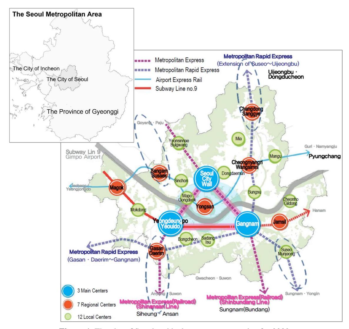
Figure 1. The city of Seoul and its long-term master plan for 2030.
We defined an urban rail station as a node and a railway network as a line and calculated the centrality index of each station using the urban network analysis tool ArcGIS. The ArcGIS tool (Sevtsuk and Mekonnen, 2012) can be used to compute five types of network analysis measures: reach, gravity, betweenness, closeness, and straightness. We selected three of these centrality measures for our analysis: reach, betweenness, and closeness. Because gravity is conceptually similar to reach, their values tend to be highly correlated. For this reason, the value of gravity was excluded from the analysis. Straightness, which indicates the gap between Euclidean distance and network distance, is useful for the analysis of buildings on a road network but is considered unsuitable for station analysis on urban rail networks. Therefore, we also excluded this indicator.
We calculated reach, betweenness, and closeness as follows. The reach measure captures how many surrounding nodes each station reaches within a given search radius in the network (Sevtsuk and Mekonnen, 2012). In other words, a station with a large value for this index has many stations located nearby. It is defined as,
\[C_i^R = \sum_{j \in G - i, d[i, j] \le r} j \tag{1}\] where \(C_i^R\): Reach value of i station
i, j: Origin (i) and destination (j) stations
G: All stations in the study area
d[i,j]: Shortest path distance between stations i and j in G
r: Radius of analysis
The betweenness of a station is defined as the fraction of the shortest paths between pairs of other stations in the network that pass through station i (Sevtsuk and Mekonnen, 2012). A station with a large value for this index is in a position where it can act as a transport hub. The betweenness measure is defined as,
\[C_i^B = \sum_{\substack{i,k \in G-i,d[i,k] \le r}} \frac{n_{jk}[i]}{n_{jk}} \tag{2}\] where \(C_i^B\): Betweenness value of i station
i, j, k: Stations
\(n_{ik}[i]\): Number of shortest paths from j to k that pass through station i
\(n_{ik}\): Total number of shortest paths from j to k
G: All stations in the study area
The closeness measure indicates how close a station is to all other surrounding stations within a given distance (Sevtsuk and Mekonnen, 2012). A station with a large value for this index is located near the center of the analysis site (Seoul). The closeness centrality is defined as,
\[C_i^C = \frac{1}{\sum_{i \in G - \{i\}, d[i,j] \le r} d[i,j]}\](3)
where \(C_i^{\mathcal{C}}[i]\): Closeness value of i station
i, j: Origin (i) and destination (j) stations
G: All stations in the study area
d[i,j]: Shortest path distance between stations i and j in G
r: Radius of analysis
Model Design
We analyzed the impact of the urban rail network centralities and the land-use characteristics of station catchment areas on the number of passengers and the average distance traveled from each station using a multivariate linear regression model. The network centralities were divided into two groups: the distance from a station to the CBD and the number of lines traversing the station (which were used in Model 1), and the reach centrality, betweenness centrality, and closeness
centrality indices (which were used in Model 2). Each model analyzed the effect on the number of passengers (Model 1-1, Model 2-1) and the average distance traveled by passengers (Model 1-2, Model 2-2). We compared the analysis results of Model 1 and Model 2 to confirm the utility of SNA. The multivariate linear regressions are expressed in the following equations,
Model 1 (1-1, 1-2): \[y_i = \alpha_0 + \beta_i D_i^{CBD} + \gamma_i N_i^{line} + \sum \delta_i L_i^l\] (4)
Model 2 (2-1, 2-2): \[y_i = \alpha_0 + \sum \beta_i C_i^k + \sum \delta_i L_i^l\] (5)
where \(y_i\): dependent variables (\(TP_i\): Model 1-1 and 2-1; \(AD_i\): Model 1-2 and 2-2); \(TP_i\): total number of passengers at station i; \(AD_i\): average travel distance from station i to all other stations; \(\alpha_0\): constant value; \(\beta_i\), \(\gamma_i\) and \(\delta_i\): parameters; \(D_i^{CBD}\): network distance from station i to CBD (Euljiro 3-ga station); \(N_i^{line}\): number of urban rail lines passing through station i; \(L_i^l\): land-use patterns (land-use characteristics) of station i's catchment area (within a [Euclidean distance of 500 m] radius from station i) l = r (residential), c (commercial), e0 (business), e1 (public), e2 (other), den (density), and div (diversity land-use); e3 (reach centrality: radius of analysis limited to 10 km), e3 (betweenness centrality: radius of analysis limited to 10 km), and e3 (closeness centrality).
The subway traffic data that was used as the dependent variable was taken from a report on the monthly passenger transport performance of the subway throughout 2011 provided by Korea Railroad (KORAIL). The independent variables were defined as the urban rail network centralities (Model 1: \(D_i^{CBD}\), \(N_i^{line}\) or Model 2: \(C_i^k\)) and the control variables were the land-use characteristics of the station catchment area (\(L_i^l\)). The shape information on urban rail lines and stations used to calculate network centrality was provided by the Korea Transport Institute (KOTI). The land-use characteristics for each urban rail station were calculated using building register data from Seoul.
The land-use pattern of the station catchment areas was calculated as the sum of residential \((L_i^R)\), commercial \((L_i^C)\), business \((L_i^B)\), public \((L_i^P)\), and other \((L_i^O)\) facilities' floor space within a radius of 500 m (Euclidean distance) from each station. The density \((L_i^{den})\) was calculated by dividing the total floor area of all buildings within a radius of 500 m (Euclidean distance) from each station into the land area of the catchment. There are two reasons why this study used only building density, not population density and activity density. The first is the multicollinearity problem. Building density is an indicator that is very close to population and activity density. Second, while the density of a building can be directly controlled through planning, population and activity cannot. In order for the results of this study to be utilized in future urban planning, it was determined that variables that the planner can directly control were appropriate. Diversity \((L_i^{div})\) was calculated by defining the catchment area for each station in the same way and measuring the mix of land use using Shannon's diversity index (SHDI) (Shannon, 1948). SHDI is widely used, and is defined as follows,
\[SHDI = -\sum_{i=1}^{N} P_i ln P_i\] (6)
where N is the number of land-use types and \(P_i\) the proportional abundance of the i-th type (Nagendra, 2002).
Table 1 presents the list of variables used in this analysis, together with their names, descriptions, and sources. The structure of the analysis model is shown in Figure 2.
Table 1. Variables and descriptions
| Division of va | ariables | Symbol | Description (unit) | Source (year) | |||
|---|---|---|---|---|---|---|---|
| Dependent variables | (Model 1-1 | 1, 2-1) | \(TP_i\) | Total number of passengers getting on and off urban rail station i in 2011 (people) | KORAIL - (2011) * | ||
| (Model 1-2 | 2, 2-2) | \(AD_i\) | Average travel distance to each urban rail station in 2011 (km) | (2011) | |||
| CBD and | \(D_i^{CBD}\) | Network distance from station i to CBD (Euljiro 3-ga station) (m) | |||||
| Network | lines (Model 1) | \(N_i^{line}\) | Number of urban rail lines at station \(i\) (EA) | - _ KOTI** | |||
| centrality | Social | \(C_i^R\) | Reach centrality value of station i | (2011) | |||
| · | network analysis (Model 2) | \(C_i^B\) | Betweenness centrality value of station i | - ` ´´ - | |||
| \(C_i^{C}\) | Closeness centrality value of station i | ||||||
| \(L_i^r\) | Total residential floor-space area in station \(i\)'s catchment area (500 m) (m2) | Seoul building | |||||
| Independent variables | \(L_i^c\) | Total commercial floor-space area in station \(i\)'s catchment area (500 m) (m2) | |||||
| I and | \(L_i^b\) | Total business floor-space area in station i 's catchment area (500 m) (m2) | |||||
| Land-use characteristics | Total public floor-space area in station \(i\)'s catchment area (500 m) (m2) | - register data - (2011) | |||||
| \(L_i^o\) | Total others floor-space area in station \(i\)'s station catchment area (500 m) (m2) | *** | |||||
| \(L_i^{den}\) | Density of all land-use floor-space area in station i's catchment area (500 m) | - | |||||
| \(L_i^{div}\) | Mixed land-use value (diversity) of station i's catchment area (500 m) | - | |||||
*Korea Railroad; **Korea Transport Institute; *** Electronic Architectural administration information system (EAIS)
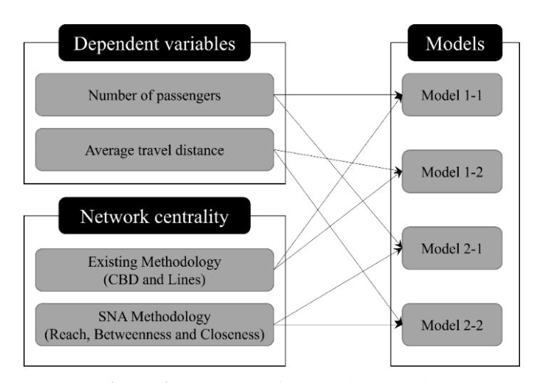
Figure 2. Structure of the analysis model.
Basic Statistics
Table 2 presents the basic statistics for each variable. The average number of passengers using Seoul urban railway stations was 7,065,536, and the average travel distance was approximately 12.45 km. The average distance from each station to the CBD station was 10.90 km, the minimum distance was 0 km, and the maximum distance was approximately 23.65 km. The reason that the minimum distance was 0 km is because that station is the CBD station itself. The average, maximum, and minimum number of urban rail lines passing through each station were 1.43 lines, 6 lines, and 1 line, respectively. Figure 3 shows the average number of passengers and the average distance for each station.
Table 2. Basic statistics
| Variables (units) | Average | SD | Maximum | Minimum | ||
|---|---|---|---|---|---|---|
| Dependent variables | Urban rail | (persons) 𝑇𝑃𝑖 | 7,065,536 | 6,405,347 | 36,403,324 | 171,190 |
| usage | (km) 𝐴𝐷𝑖 | 12.45 | 1.93 | 22.55 | 8.07 | |
| Network | 𝐶𝐵𝐷 (m) 𝐷𝑖 | 10,899.97 | 5,351.23 | 23,651.31 | 0.00 | |
| centrality (Model 1) | 𝑙𝑖𝑛𝑒 (EA) 𝑁𝑖 | 1.43 | 0.77 | 6 | 1 | |
| Network centrality (Model 2) | 𝑅 𝐶𝑖 | 77.57 | 29.82 | 126.00 | 16.00 | |
| 𝐵 𝐶𝑖 | 385.11 | 337.79 | 1,840.00 | 0.00 | ||
| 𝐶 𝐶𝑖 | 8.472E-08 | 8.936E-09 | 9.69369E-08 | 6.30521E-08 | ||
| Independent | 𝑟 𝐿𝑖 (m2) | 582,567.46 | 362,364.94 | 2,658,406.12 | 0.00 | |
| variables | 𝑐 𝐿𝑖 (m2) | 250,594.38 | 282,320.61 | 2,526,286.11 | 263.52 | |
| 𝑏 (m2) 𝐿𝑖 | 204,691.61 | 353,035.61 | 2,387,842.12 | 0.00 | ||
| Land-use characteristics | 𝑝 (m2) 𝐿𝑖 | 93,540.56 | 98,357.80 | 699,516.25 | 355.68 | |
| 𝑜 (m2) 𝐿𝑖 | 43,873.71 | 43,585.15 | 231,846.56 | 686.40 | ||
| 𝑑𝑒𝑛 𝐿𝑖 | 170.71 | 66.30 | 513.81 | 23.11 | ||
| 𝑑𝑖𝑣 𝐿𝑖 | 1.052 | 0.28 | 1.55 | 0.22 |
SD, Standard Deviation
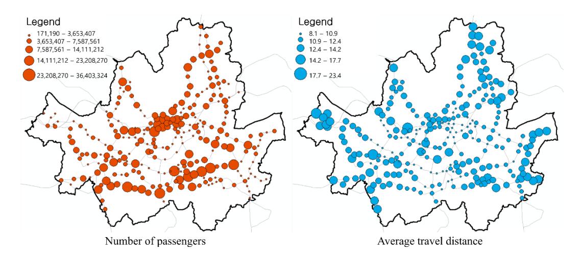
Figure 3. Dependent variables.
The network centrality for each station was calculated using SNA. The radius of analysis for reach and betweenness was limited to 10 km because there was no significant difference between using 10 km and 12.44 km. However, the radius for closeness was not limited to the analysis, because closeness was also used to analyze the spatial proximity to all nodes in the analysis area. As no limiting radius was imposed, stations located closer to the center of the graph obtained higher closeness values (Sevtsuk and Mekonnen, 2012). The average reach, betweenness, and closeness were 77.57, 385.11, and 8.472 × 10⁻⁸, respectively. For easy understanding of the various topologies for each station, the maps for each network centrality index are shown in Figures 4-6.
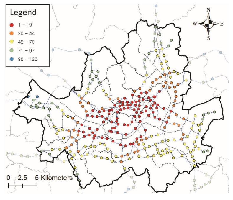
Figure 4. Estimated reach value in Seoul.
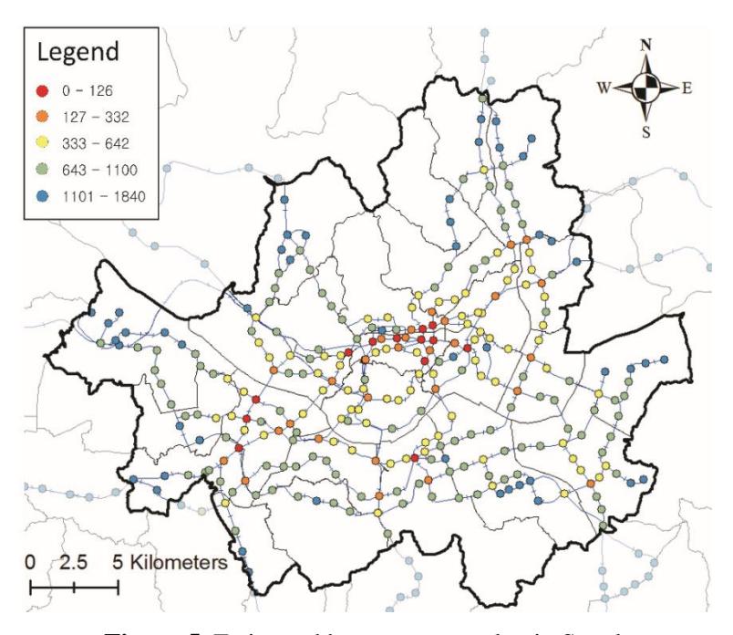
Figure 5. Estimated betweenness value in Seoul.
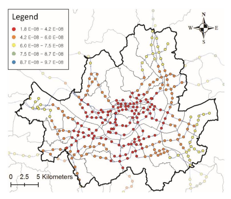
Figure 6. Estimated closeness value in Seoul.
The reach centrality index is the number of stations in the analysis range for each station. This index is high in areas where urban stations are clustered. (Figure 4). The betweenness centrality index indicates the linkage with other stations in the analysis range for each station. The results of the calculation showed high levels for transfer stations (Figure 5). The closeness centrality indicates the proximity to the stations in all regions of the analysis area (in this study, Seoul).
High values for this index were obtained for stations in the downtown area, and low values were obtained for stations in the outskirts of the city (Figure 6). Stations located in the center of the city, but outside of the cluster, had relatively low reach centrality index values. However, the closeness value was high when a station was in the center of the city, regardless of the cluster area, and was low for stations in the outskirts of the city. The data classification method of the centrality index maps (Figure 4, 5, and 6) used natural breaks to maintain homogeneity within the same class and to maximize heterogeneity between classes.
Results and Discussion
Prior to the analysis, we verified the normality of the variables by using scatter plots. Seven variables (commercial, business, public and others floor-space area, density, number of passengers, and travel distance) showed non-normal distributions. To ensure homoscedasticity in the regression, we used natural log transformations for these variables. The results of the regression models are presented in three parts: first, Model 1 uses usual centrality; second, Model 2 uses the SNA centrality measures; finally, we compared the two sets of results. Using SNA to measure network centrality led to an improvement in the explanatory power of the regression models of the number of passengers and average travel distance for each urban rail station. A more detailed interpretation of each analysis result follows below.
Effects of Land-use Characteristic and Usual Network Centrality (Model 1)
Table 3 presents estimates of the effects of land-use characteristics and usual network centrality on the number of passengers (Model 1-1) and their average travel distance (Model 1-2). The adjusted 2 values for Model 1-1 and Model 1-2 were 0.386 and 0.268, respectively. Variance inflation (VIF) is used to measure how much the variance of the estimated regression coefficient is inflated if the independent variables are correlated. VIF is calculated as follows:
\[VIF = \frac{1}{1 - R^2} = \frac{1}{Tolerance} \tag{7}\] where, the tolerance is simply the inverse of VIF.
The lower the tolerance, the more likely is the multicollinearity among the variables. A VIF value of 1 indicates that the independent variables are not correlated to each other. The VIF criteria for determining whether multicollinearity is present are different for each researcher. However, in most studies, the threshold value to deviate small from large is generally taken as 10 (Alin, A. (2010); Senaviratna, N. A. M. R., & Cooray, T. M. J. A. (2019); Kroll, C. N., & Song, P. (2013)). As a result of the analysis, the VIF value was derived below 10, so we judged that multicollinearity did not exist.
In Model 1-1, the distance to the CBD from each station had a significant positive effect on the number of passengers and a significant positive effect on the average travel distance using an urban rail line, which was almost four times greater. The estimate for number of lines at the station (0.198) was similar to the result for distance to the CBD (0.211).
| Model 1 | Independent variables | ||||||||||
|---|---|---|---|---|---|---|---|---|---|---|---|
| Number of passengers (ln) (Model 1-1) | Ave | Average travel distance (ln) (Model 1-2) | |||||||||
| β | t | t p | β | t p | |||||||
| (Constant) | - | *** | 6.882 | 0.000 | - | *** | 11.885 | 0.000 | - | ||
| Network centrality (Model 1) | \(D_i^{CBD}\) | 0.131 | ** | 2.420 | 0.016 | 0.526 | *** | 8.892 | 0.000 | 1.274 | |
| \(N_i^{line}\) | 0.198 | *** | 4.036 | 0.000 | 0.211 | *** | 3.936 | 0.000 | 1.047 | ||
| \(L_i^r\) | -0.108 | * | -1.764 | 0.079 | -0.135 | ** | -2.018 | 0.045 | 1.633 | ||
| \(L_i^c(\ln)\) | 0.478 | *** | 5.605 | 0.000 | 0.041 | 0.444 | 0.657 | 3.158 | |||
| \(L_i^b(\ln)\) | 0.079 | 0.767 | 0.444 | -0.174 | -1.553 | 0.122 | 4.576 | ||||
| Land-use character | \(L_i^p(\ln)\) | 0.090 | 1.456 | 0.147 | 0.054 | 0.807 | 0.420 | 1.658 | |||
| istics | \(L_i^o(\ln)\) | 0.188 | *** | 2.954 | 0.003 | 0.159 | ** | 2.293 | 0.023 | 1.752 | |
| Liden (ln) | 0.054 | 0.746 | 0.456 | 0.073 | 0.916 | 0.361 | 2.293 | ||||
| \(L_i^{div}\) | -0.170 | * | -1.769 | 0.078 | -0.083 | -0.789 | 0.431 | 3.999 | |||
| \(R^2\) (Adj. \(R^2\)) | 0.406 ( | 0.386) *** | 0.293 | (0.268) *** | - | ||||||
Table 3. Results of multivariate linear regression analysis for Model 1
In terms of the land-use characteristic variables, in Model 1-1, the commercial facilities' floor space \((L_i^c)\) was highly significant (t-value = 5.605); business facilities' floor space \((L_i^b)\) was also highly significant. However, residential facilities' floor space \((L_i^r)\) had a negative effect on the number of passengers; although the t-value was small (-1.764), it had a positive effect on average travel distance. The results of this study show some differences with previous ones. While prior work found that density increased the number of station users (Cervero and Kockelman 1997; Cervero and Murakami 2009; Lin and Shin 2008), its effect was not significant here. In addition, the diversity index had a negative effect on the number of reverse users. This could mean either that the density and diversity variables may not be significant for each city to be studied or that it is necessary to calculate the topological relationship of urban railway stations more accurately.
Effects of Land-use Characteristic and Social Network Centrality (Model 2)
Before performing analysis of Model 2, multicollinearity was verified. When examining multicollinearity, we first look at the correlation between independent variables; if the value is high, multicollinearity is suspected. At this time, although opinions differ among scholars, it is common to doubt about 0.8 or higher (Shin et al., 2008; Midi et al., 2010).
When the correlation of the independent variables used in this study was calculated, the value between reach value and closeness value was calculated to be 0.772, which is relatively high (see Table 4). However, a high correlation coefficient does not necessarily mean that multicollinearity exists (Park, 2019). Therefore, multicollinearity is finally determined by looking at the VIF value.
***p < 0.01, **p < 0.05, *p < 0.1
If the VIF value is greater than 10, multicollinearity should be suspected (Alin, A. (2010); Senaviratna, N. A. M. R., & Cooray, T. M. J. A. (2019); Kroll, C. N., & Song, P. (2013)). As a result of checking the VIF values of the data used in this study, the VIF values of all variables were calculated to be less than 10 (see Table 5). After synthesizing the contents of previous studies and the analysis results of this study, we judged that the independent variable of Model 2 did not have a major problem with multicollinearity.
Table 4. Correlation between independent variables
| \(C_i^R\) | \(C_i^B\) | \(C_i^C\) | \(L_i^r\) | \(L_i^c\) | \(L_i^b\) | \(L_i^p\) | \(L_i^o(\ln)\) | \(L_i^{den}\) | \(L_i^{div}\) | |
|---|---|---|---|---|---|---|---|---|---|---|
| \(c_i\) | \(c_i\) | \(c_i\) | \(L_{\dot{l}}\) | (ln) | (ln) | (ln) | \(L_i\) (III) | (ln) | \(L_{\hat{l}}\) | |
| \(C_i^R\) | 1.000 | -0.545 | -0.773 | 0.095 | 0.161 | -0.236 | 0.078 | 0.189 | 0.245 | 0.066 |
| \(C_i^B\) | -0.545 | 1.000 | 0.196 | -0.173 | -0.075 | 0.041 | 0.093 | 0.048 | -0.080 | -0.154 |
| \(C_i^c\) | -0.773 | 0.196 | 1.000 | 0.091 | -0.199 | 0.224 | -0.246 | -0.373 | -0.244 | -0.001 |
| \(L_i^r\) | 0.095 | -0.173 | 0.091 | 1.000 | -0.159 | -0.100 | -0.124 | -0.146 | 0.048 | 0.453 |
| \[\frac{L_i^c}{(\ln)}\] | 0.161 | -0.075 | -0.199 | -0.159 | 1.000 | -0.384 | -0.328 | 0.002 | -0.287 | -0.148 |
| \(\frac{L_i^b}{(\ln)}\) | -0.236 | 0.041 | 0.224 | -0.100 | -0.384 | 1.000 | 0.239 | -0.024 | -0.387 | -0.532 |
| \(L_i^p\) (ln) | 0.078 | 0.093 | -0.246 | -0.124 | -0.328 | 0.239 | 1.000 | 0.120 | -0.350 | -0.319 |
| \[\frac{L_i^o}{(\ln)}\] | 0.189 | 0.048 | -0.373 | -0.146 | 0.002 | -0.024 | 0.120 | 1.000 | -0.320 | -0.325 |
| Liden (ln) | 0.245 | -0.080 | -0.244 | 0.048 | -0.287 | -0.387 | -0.350 | -0.320 | 1.000 | 0.543 |
| \(L_i^{div}\) | 0.066 | -0.154 | -0.001 | 0.453 | -0.148 | -0.532 | -0.319 | -0.325 | 0.543 | 1.000 |
In Model 2, we used SNA measures of centrality and tested their effects on the number of passengers and average travel distance (Table 5). Not only were more variables significant but also the explanatory power of the regression model increased. All of the network centrality variables, including reach \((C_i^R)\), betweenness \((C_i^B)\), and closeness \((C_i^C)\), were significant predictors of the number of passengers. Reach and closeness variables were also significant predictors of average travel distance. A more detailed interpretation of each analysis result follows.
The network centrality variables were important in explaining the number of passengers at urban rail stations. The most significant variable among them was reach \((C_i^R)\); it had a negative standardised coefficient, such that higher reach \((C_i^R)\) decreased the number of passengers. When there were more alternative stations available around one station, fewer passengers used the station. The coefficients of closeness \((C_i^C)\) and betweenness \((C_i^R)\) were positive, showing an increase in passengers when closeness \((C_i^C)\) and betweenness \((C_i^B)\) increased. Based on these results, the number of passengers increases when the station is connected to several lines or located near the city center. This study went a step further than Gonçalves et al. (2009) by empirically analyzing the effects of the network centrality categories.
The reach variable \((C_i^R)\) had a significant negative effect on the average travel distance; its coefficient (-0.727) and t-value (-6.885) were the highest among the network centrality variables. Betweenness \((C_i^B)\) was not significant, meaning that the network centrality of an urban railway is not related to a decreased travel distance. The closeness \((C_i^C)\) was also significant; its coefficient (0.329) and t-value (3.150) indicated a positive effect on average travel distance.
Higher reach values indicate that there are more stations that can be used as origins and destinations. For this reason, as the reach value increases, the average travel distance decreases. Stations with a large closeness value are in the center of the city. At stations with large values, the average distance of travel is longer. The results of this analysis are deeply related to the urban spatial structure of the Seoul metropolitan area. The social, economic, and cultural facilities of the Seoul metropolitan areas (Seoul, Gyeonggi, and Incheon) are concentrated in the center of Seoul, where the closeness value is high. In addition, residences are concentrated in the suburbs of Seoul, Gyeonggi, and Incheon. This urban spatial structure causes long-distance traffic for people who make Seoul's center a destination for their activities.
These results contradict the results from Model 1, which used the distance from the CBD as an independent variable. Unlike Model 1, Model 2 used the SNA reach value as control. In other words, the distances to the CBD used in Model 1 constitute a mixture of the reach value and the closeness value calculated through SNA. Hence, the model's explanatory power was diminished.
In terms of the land-use characteristic variables, business facilities' floor space \((L_i^b)\) had a significant negative effect on average travel distance. Public facilities' floor space \((L_i^p)\) and density of all land-use floor space \((L_i^{den})\) had significant positive effects on number of passengers and average travel distance. These results contrast with the results in Table 3 discussed above. As with the various previous studies presented above (Cervero and Kockelman, 1997; Cervero and Murakami, 2009; Lin and Shin, 2008), the density variable had a positive effect on average distance traveled by users of the subway station. Diversity had a negative effect on number of users in urban train stations, as in previous studies in Korea (Sung et al, 2014; Yoo, 2013). Additionally, the significance of most land-use variables compared to Table 3 indicates that application of the SNA methodology used in this study was important.
Table 5. Results of multivariate linear regression analysis for Model 2
| Independent variable | ||||||||||
|---|---|---|---|---|---|---|---|---|---|---|
| Model 2 | Number of passengers (ln) | (Model 2-1) | Average travel distance (ln) (Model 2-2) | VIF | ||||||
| β | t | p | β | t | p | |||||
| (Constant) | -*** | 3.413 | 0.001 | -*** | 6.895 | 0.000 | - | |||
| 𝑅 𝐶𝑖 | -0.551*** | -6.382 | 0.000 | -0.727*** | -6.885 | 0.000 | 5.877 | |||
| Network centrality (Model 2) | 𝐵 𝐶𝑖 | 0.225*** | 4.477 | 0.000 | -0.023 | -0.368 | 0.713 | 2.001 | ||
| 𝐶 𝐶𝑖 | 0.397*** | 4.662 | 0.000 | 0.329*** | 3.150 | 0.002 | 5.740 | |||
| 𝑟 𝐿𝑖 | -0.154*** | -3.515 | 0.001 | -0.128** | -2.379 | 0.018 | 1.515 | |||
| 𝑐 (ln) 𝐿𝑖 | 0.449*** | 6.195 | 0.000 | 0.137 | 1.542 | 0.124 | 4.158 | |||
| 𝑏 (ln) 𝐿𝑖 | -0.080 | -1.030 | 0.304 | -0.381*** | -4.022 | 0.000 | 4.737 | |||
| Land-use characteristics | 𝑝 (ln) 𝐿𝑖 | 0.147*** | 2.764 | 0.006 | 0.187** | 2.873 | 0.004 | 2.234 | ||
| 𝑜 (ln) 𝐿𝑖 | 0.227*** | 4.409 | 0.000 | 0.276*** | 4.371 | 0.000 | 2.100 | |||
| 𝑑𝑒𝑛 𝐿𝑖 (ln) | 0.160** | 2.468 | 0.014 | 0.351*** | 4.425 | 0.000 | 3.322 | |||
| 𝑑𝑖𝑣 𝐿𝑖 | -0.173** | -2.473 | 0.014 | 0.014 | 0.168 | 0.867 | 3.849 | |||
| 2 2 𝑅 (Adj. 𝑅 ) | 0.671 (0.658) *** | 0.507 (0.488) *** | - | |||||||
***p < 0.01, **p < 0.05, *p < 0.1
Effects of Improvements
Finally, we summarize the improvements secured by using SNA to determine network centrality (see Table 6). For an explanation of the number of passengers, the adjusted 2 showed an improvement of 0.272 (from 0.386 to 0.658) and the number of significant variables increased from six to nine when we applied SNA. For the model of the average travel distance, the adjusted 2 showed an improvement of 0.220 (from 0.268 to 0.488) and the number of significant variables increased from four to seven when we applied SNA. These improved results indicate that models using network centrality variables created through SNA can better explain the number of passengers and the average travel distance by as much as 27.2% and 22.0%, respectively. Moreover, these results show that social network centrality is better than the usual network centrality in determining which variables increase the number of passengers and decrease the average travel distance. In addition, increasing the number of significant variables implies that we can formulate more methods for increasing the number of passengers or decreasing the average travel distance.
| Models | Dependent variables | 2 2 𝑅 (Adj. 𝑅 ) | No. of significant variables | |
|---|---|---|---|---|
| Model 1-1 | Number of passengers (ln) | 0.406 (0.386) | 6 | |
| Model 1 | Model 1-2 | Average travel distance (ln) | 0.293 (0.268) | 4 |
| Model 2-1 | Number of passengers (ln) | 0.671 (0.658) | 9 | |
| Model 2 | Model 2-2 | Average travel distance (ln) | 0.507 (0.488) | 7 |
| Improvement (Model 2 – Model 1) | Number of passengers (ln) | +0.265 (0.272) | +3 | |
| Average travel distance (ln) | +0.214 (0.220) | +4 | ||
Table 6. Comparison of improvements between Model 1 and Model 2
Conclusions
TOD has become one of the key planning methods to manage urban growth intelligently in the twenty-first century. In the academic world, research on constructing a theoretical framework for TOD definition, characteristics, and design guidelines, as well as empirical studies for predicting the effect of TOD implementation have been conducted. However, analyses of the catchment areas have emphasized flaws in how the topology of stations has been measured.
This study shows the applicability of the SNA technique in urban planning. Although SNA was developed for social networks, it has recently also been applied in urban research, e.g., for geographical analysis and transportation planning. In the field of urban planning, SNA has been implemented using road networks to calculate regional centrality indexes, which is used to determine urban spaces or activities. This study extended the coverage of SNA from road networks to public transportation networks. The centrality of each station was used for analysis of the catchment area. Thus, this research provides an opportunity to apply the same methodology not only to the physical network of a city but also to public transport routes or vehicle travel paths.
Secondly, we proposed an application of this method to the calculation of the topology of stations in TOD analysis. Studies of TOD have proposed and implemented many different methodologies for quantifying the topology of stations. However, as explained above, these approaches have several limitations. We presumed that SNA could be an alternative to overcome these limitations. The centrality of a station computed using SNA provides not only a quantitative measurement of the number of links passing through a station but also the relationship with nearby stations and, by extension, the topology of each station within the entire city. Using this centrality measure in the analysis of the catchment area of a station overcomes the limitations of prior TOD studies.
Thirdly, we analyzed the factors affecting the number of passengers as well as the travel distance. It was emphasized that the transportation service quality should be increased for sustainable urban development not only in the field of TOD but also in other urban planning areas. Based on this paradigm, numerous studies have been conducted to identify factors that affect the number of users of public transit. However, it is necessary to increase the number of users and shorten the travel distance to utilize the limited public transportation infrastructure efficiently. Reducing the distance traveled by urban rail users contributes to lowering the number of passengers on carriages. This reduces the congestion of carriages, which increases the quality of service of transportation. This study is meaningful in that it addresses the issue of travel distance, which has been neglected in previous studies despite its contribution to improving public transportation utility.
These three contributions make this study academically meaningful and provide significant benefits towards determining policies related to public transit. Previous studies had two limitations. Firstly, there were limitations regarding how station topology was calculated. Existing studies (Lee et al., 2013; Lyu et al., 2016; Nasri and Zhang, 2014; Arrington and Cervero, 2008; Sohn and Shim, 2010; Jun et al., 2015) did not reasonably calculate station topology. This study is significant in that station topology was rationally derived by applying the SNA methodology. Secondly, existing studies (Cervero, 1996; Cervero and Kockelman, 1997; Ewing and Cervero 2001; Cervero and Murakami 2009; Lin and Shin 2008; Sung et al 2014; Yoo 2013) mainly analyzed factors affecting the increase in the number of passengers. As the number of passengers increases, the efficiency of public transport increases, but the quality-of-service decreases (MVA Consultancy, 2008; Kato, 2014). Therefore, this study is meaningful in that it included the travel distance of passengers, which affects the congestion of passenger cars, in the analysis.
This study confirmed that the supply of new subway lines could change the topology of existing subway stations, which could also affect existing passenger traffic patterns. This study provides an indicator for measurement of how the traffic patterns of existing urban rail users will change with the supply of new routes. This means that this empirical study can greatly contribute to public transportation policymaking. In future studies, we will assess how changes in centrality due to the expansion of urban railway routes affect the number of passengers and traffic distance. In a follow-up study, we will perform the same analysis based on recent data and compare the analysis results with 2011 data to verify the difference.
Acknowledgments
This study was conducted with the support of the Korea Agency for Infrastructure Technology Advancement. (22CTAP-C164289-02).