
Introduction
Cities host more than half of the world's population since the turn of the century and will be home to almost seven out of ten people by 2050 (United Nations 2019). The networks of urban roads historically came first and remain to be the main transportation channels for these cities (Uhl et al. 2022). With the continuous growth of the urban population and the geospatial constraints in growing urban zones, the road network systems are increasingly put under immense pressure, leading to congestion and the associated deleterious effects on the economy (Sweet 2011) and the well-being of the general population (Smyth et al. 2008, Yin & Shao 2021). Because of this, the study of street network architecture is deemed to be important and timely. It is usually framed from the perspective of human livability (Ahmed et al. 2019), but this approach is deemed rather primitive, being based on the point of view of a person living within the larger scale of the city road network architecture.
Another equally fruitful and important approach is to view the system from the outside, i.e., looking at the streets from a bird's eye view. In particular, one can view the entire road network as a single system whose collective behavior can be measured and analyzed (Batty, 2000; Lämmer et al., 2006; Xie & Levinson, 2007; Barthelemy et al., 2013; Masucci et al., 2013). Such studies are made possible by the availability of detailed geographical information system (GIS) data (Nguyen et al., 2014) along with satellite imagery and other surveying techniques (Puente et al., 2013). Of course, viewing a simple snapshot of a road network may reveal complex properties that are qualitatively different from one city to another; there is a need for robust quantitative characterizations to extract relevant metrics for further analyses. These quantitative approaches not only describe the streets as currently constituted but also model the origins and the evolution of the road network (Courtat et al., 2011) and aim to find their associated effects on other urban elements (Porta et al., 2012).
One of the most straightforward ways of quantifying a road network layout over geographical space involves a statistical characterization of the shapes formed by the roads on the ground (Lämmer et al., 2006; Cirunay & Batac, 2018). These characterizations quantify the within-city morphologies generated by the construction of roads. Another straightforward and useful tool is fractal analysis (Batty & Longley, 1994). While fractals were first used on natural formations (Mandelbrot, 1982), it has found application with respect to other complex formations in human society, particularly on road networks (Frankhauser, 1998; Zhang & Li, 2012; Chen, 2013). Fractal analysis offers a distinct advantage as a characterization tool, as it naturally incorporates the road cover and spatial configurations found in road networks into a single metric, the fractal dimension δ. An even higher level of analysis involves viewing road networks from the theory of space syntax (Hillier & Hanson, 1984; Hillier, 1996), which not only accounts for the spatial arrangement but also the network connectivity of roads, and their associated effects on other elements of the built environment and on human activity (Hillier, et al. 1993; Penn et al., 1998). These approaches have been used successfully to quantitatively describe urban typologies of representative cities in Europe (Berghauser Pont et al., 2019; Paraskevopoulos & Bakogiannis, 2022) and North America (Smart et al., 2020), clearly illustrating their similarities and differences and describing their effects on human activity and mobility (Bobkova et al., 2019). When taken together, these analytical tools allow for quantitative comparisons between city road networks and provide metrics for use in designing effective management and further development strategies.
In this paper, we present a fundamental characterization based on the statistical distributions of geometrical metrics and fractal analysis for quantifying the morphologies created by roads in representative component cities and municipalities in the Philippines. It focuses on the metropolitan centers of urbanization and economic growth in the three main island groups in the country: Metro Manila, Metro Cebu, and Metro Davao. By combining fractal analysis with the statistics of dimensionless shape metrics of roads and road-bounded blocks, we obtained insights regarding the state of the road architecture. Here, we highlight the differences in terms of economic conditions and geographical constraints. This is important because it adds to the growing literature on complex system approaches to urban systems, in particular, cities in archipelagic settings such as the Philippines.
Background and Framework
Urban systems as complex systems
The foundation for complex systems research in the physical sciences is usually attributed to Anderson, who proposed a perspective for understanding things that show emergent properties (Anderson, 1972). He recognized that many of the properties attributed to materials cannot be used to describe the individual constituents; for example, while gold is metallic (and malleable, a good conductor, etc.), a single gold atom is most definitely not. Anderson thus coined the phrase "more is different" to frame the study of complex systems in the physical world (Anderson, 1972). In the subsequent decades, and with the availability of faster computational tools and better data collection, scientists, particularly physicists, have begun uncovering more examples of complex phenomena in nature, computer models, and human society, among others (Sherrington, 2010), culminating in the descriptive phrase "the whole is more than the simple sum of its parts" (Gell-Mann, 2002). Subsequently, the principles of complex systems analysis have been applied to road networks and other urban attributes (Batty, 2000).
Road networks, in particular, are very good examples of the emergence of complexity in urban systems. The actual layout of a road network is a complex pattern, one that has emerged out of centuries of local development. Save for a few examples of completely planned cities from the top down (Wigmore, 1972; Vernon, 2006; Batista et al., 2006), or smart cities built from scratch (Loo & Tang, 2019), most cities have originated from self-organization, i.e. dictated by local conditions on the ground and thus exhibiting bottom-up emergent mechanisms. Previous works have identified local rules for road creation operating at various stages in a city's development (Strano et al., 2012). Earlier stages involve exploratory mechanisms that create long, sinuous roads for the main purpose of connectivity with other regions. As the city matures, it operates based on homogenization, i.e., subdividing the available space into regular, equitable blocks, resulting in a densified network. Despite the simplicity of these underlying rules, the actual geographical and socio-economic conditions give rise to the rich patterns of road network imprints (Cirunay & Batac, 2020).
Measuring spatial complexity
The complexity of urban spatial extent has been gauged based on different metrics and criteria. For example, early works used cellular automata modeling to replicate the spatial patterns of cities (Makse et al., 1995). Cellular automata (CA) models are good representative systems for illustrating emergence, due to the complex patterns that emerge out of simple local rules; the fact that urban imprints have been replicated using CA shows that they are, indeed, large-scale complex systems (Batty, 2005). In works that specifically analyzed road networks, previous
authors used fractal analysis to understand road cover and structure (Batty & Longley, 1994; Murcio et al., 2015; Cirunay & Batac, 2018). As expected, as the road networks evolve in complexity and fill the available space, the street patterns evolve from a multi-fractal to a monofractal structure (Murcio et al., 2015). Fractal analysis therefore quantifies the different spatial and temporal conditions within and among cities.
Another class of spatial analysis focuses on the statistical distributions of the morphological entities created by roads in space (Louf & Barthélemy, 2014). Apart from being straightforward one just needs to collect the shapes and measure them—this approach has been shown to produce emergent signatures that can be observed for a wide class of city behavior. Whether applied to cities from the global north (Lämmer et al., 2006; Masucci et al., 2009) versus those from the global south (Cirunay & Batac, 2018), or in planned versus organically grown conditions (Cirunay & Batac, 2021); and even in urban versus rural settings (Strano et al., 2017), the statistical distributions of the city road network morphologies follow nearly universal characteristics. Most of these distributions are highly skewed to the right with tails that exhibit power-law scaling (Lämmer et al., 2006; Cirunay & Batac, 2018).
In this work, the spatial complexity of road networks spread over urban areas was analyzed using dimensionless shape factors and fractal analyses. This is one of the first examinations of this kind applied to the archipelagic setting of the Philippines, where economic and urban growth is disproportionately biased towards the capital at the expense of other regional centers. The shape factor and fractal analyses conducted on geographical information system (GIS) data presents an interface between the natural and mathematical (physics and mathematics), computational (data science and complexity), and social and economic (urban planning and development) sciences, paving the way for multidisciplinary approaches geared towards more efficient urban management and planning.
Materials and Methods
Metropolitan regions of the Philippines
The Philippines is an archipelagic country composed of more than 7,000 islands. The Philippine government has classified three metropolitan centers across the three major island groups that act as gateways for economic activity in these regions (NEDA, 2017). The Metro Manila conurbation on the island of Luzon is the most populous urban conurbation and is also the National Capital Region (NCR) of the Philippines. The Metro Cebu area serves as the regional gateway for the Visayas group of islands. At the southern island of Mindanao, the Metro Davao conurbation has the largest land area of the three. Due to data completeness and accuracy issues, we were only able to obtain a subset of all the cities and municipalities comprising these metropolitan agglomerations. Figure 1 shows the geographical locations of these metropolitan regions, and their relative scales.
The geographical locations of the metropolitan regions shown in Figure 1 makes them good representative cases for comparing the level of complexity of the urban road networks in different regional centers of the Philippines. The Metro Manila conurbation (blue boxed region in Figure 1), being the National Capital Region (NCR) of the Philippines, has the densest road network, in part due to its smaller total area. Despite this, the capital region has the highest population and is the main contributor to the economic activity of the country. The Metro Cebu area (green boxed region in Figure 1) is in the center of the Philippines and is the major urban gateway for the Visayas group of islands. Finally, the Metro Davao area (red boxed region in Figure 1) is in southeastern Mindanao, the most southern group of islands in the Philippines. Davao City, which is the central hub of the conurbation, is the largest city in the Philippines in terms of land area; the Metro Davao region is also the largest conurbation among the three city groups considered.
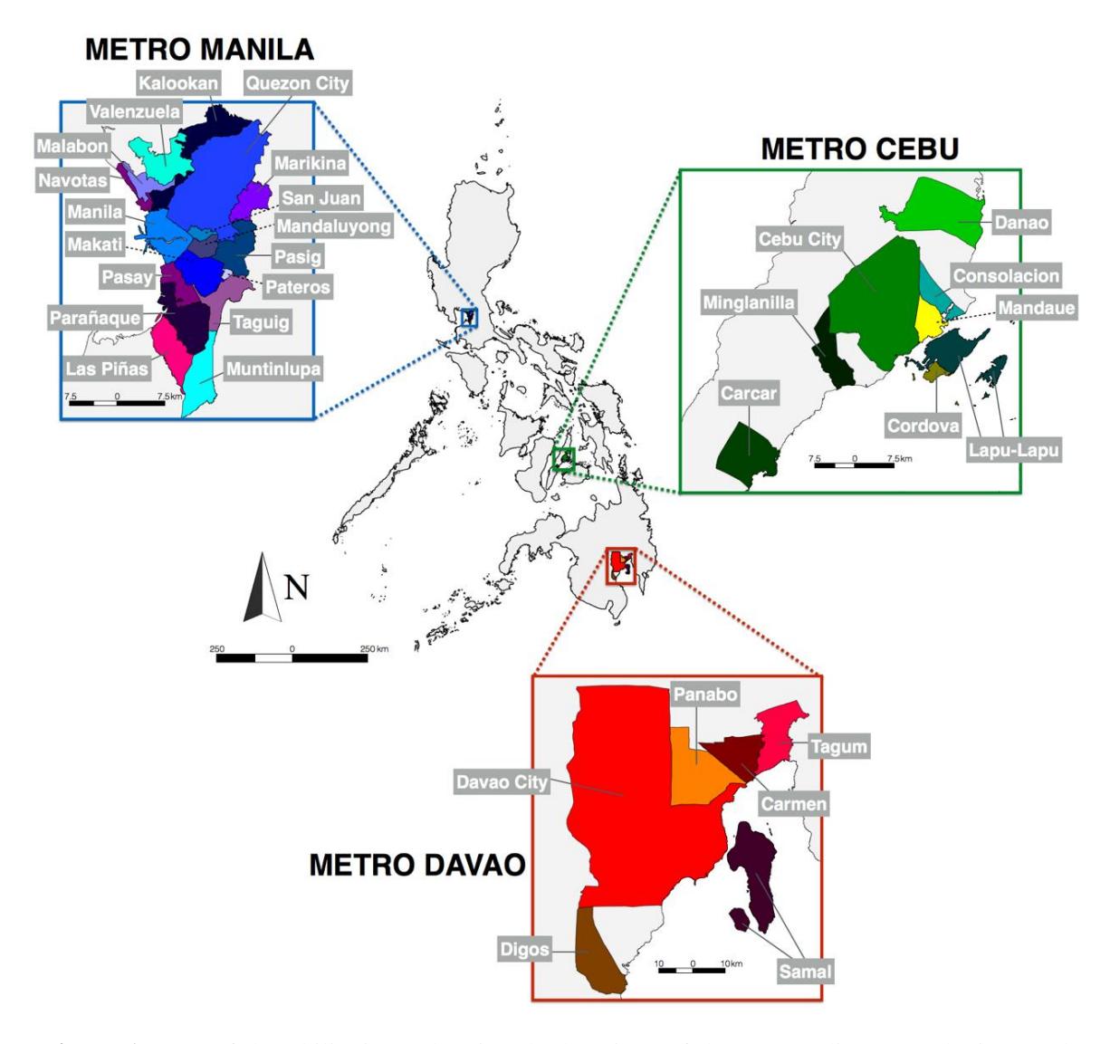
Figure 1. Map of the Philippines, showing the locations of the metropolitan conurbations and representative cities and municipalities considered in this work. The Metro Manila conurbation (blue boxed region) on the northern island of Luzon is the National Capital Region (NCR) of the Philippines. The Metro Cebu conurbation (green boxed region) is located in the Central Philippines. The Metro Davao (red boxed region) is located on the southern island of Mindanao.
Table 1 below shows the properties of the conurbations and the component units considered in this work. Again, due to data completeness issues, some component cities and municipalities in Metro Cebu and Metro Davao were not included in the analyses. Only the properties of the cities and municipalities included in the study are presented in the tabulation.
Table 1. Philippine metropolitan centers and constituent units considered
| Unit | Land area (km2)a | Populationb |
|---|---|---|
| Metro Manila | 619.57 | 13,484,462 |
| Caloocan | 55.80 | 1,661,584 |
| Las Piñas | 32.69 | 606,293 |
| Makati | 21.57 | 629,616 |
| Malabon | 15.96 | 380,522 |
| Mandaluyong | 21.26 | 425,758 |
| Manila | 38.55 | 1,846,513 |
| Marikina | 21.52 | 456,059 |
| Muntinlupa | 38.75 | 543,445 |
| Navotas | 10.77 | 247,543 |
| Parañaque | 47.69 | 689,992 |
| Pasay | 13.97 | 440,656 |
| Pasig | 31.00 | 803,159 |
| Pateros* | 1.76 | 63,643 |
| Quezon City | 161.11 | 2,960,048 |
| San Juan | 0.23 | 126,347 |
| Taguig | 53.67 | 886,722 |
| Valenzuela | 47.02 | 714,978 |
| Metro Cebu | \[\textbf{1,062.88}^{\dagger}\] | \[3{,}165{,}799^\dagger\] |
| Carcar | 116.78 | 136,453 |
| Cebu City | 315.00 | 964,169 |
| Consolacion* | 37.03 | 148,012 |
| Cordova* | 17.15 | 70,595 |
| Danao | 107.30 | 156,321 |
| Lapu-Lapu | 58.10 | 497,604 |
| Mandaue | 34.87 | 364,116 |
| Minglanilla* | 65.60 | 151,002 |
| Metro Davao | 6,492.84† | 3,339,284† |
| Carmen* | 166.00 | 82,018 |
| Davao City | 2,443.61 | 1,776,949 |
| Digos | 287.10 | 188,376 |
| Panabo | 251.23 | 209,230 |
| Samal | 301.30 | 116,771 |
| Tagum | 195.80 | 296,202 |
<sup>a</sup> Land area figures are from the Philippine Statistics Authority 2015 Census (PSA 2015)
The road network GIS data for the representative cities were obtained from OpenStreetMap (OSM, n.d.), an online mapping platform that takes in data contributed by users. As expected, the different regions show different completeness levels due to the different levels of user reporting (Orden et al., 2020; Thinking Machines Data Science, n.d.). For the cities and municipalities considered in Table 1, however, the historical and main roads are well represented.
The road networks were obtained as sets of nodes with coordinates \((\phi, \theta)\), where the longitude \(\phi\) and latitude \(\theta\) are reported in degrees. Each node represents an intersection, fork, bend, or other important location in space deemed important by the cartographer. A contiguous road, denoted by a unique number, r, is represented as a set of node coordinates \((\phi_r, \theta_r)\) arranged in order of traversal. The OSM road network data was processed using QGIS and intersected with the political boundaries of the city or municipality under consideration.
<sup>b</sup> Population figures are from Philippine Statistics Authority 2020 Census (PSA 2020)
* Municipality; not a chartered city.
† Figure includes data from other cities/municipalities in the conurbation not included in this study
Dimensionless morphological metrics
Two prevalent morphological forms (shapes) can be extracted from the network of city streets. One can obtain the actual roads or the road-bounded areas or blocks they form. Previous works have shown that the statistical distributions of the road lengths and block areas follow heavytailed distributions spanning several orders of magnitude (Lämmer et al., 2006; Masucci et al., 2013; Cirunay & Batac, 2018). Despite the huge differences in scale, previous works have introduced dimensionless metrics that allow for a common characterization despite differences in size (Cirunay & Batac, 2018; Cirunay & Batac, 2021). Figure 2 illustrates these metrics and how their representative values are observed in space.
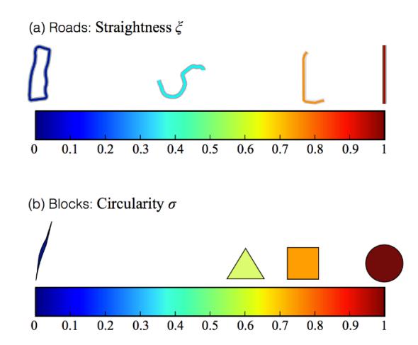
Figure 2. Illustrating the Morphological Metrics' Representative Values. (a) The straightness is a normalized dimensionless metric for roads: closed roundabouts have = 0 while straight roads have = 1. Other noteworthy cases involve the case of = 1/, when the road follows the sinuosity of the terrain; and ≈ 0.6 − 0.8, for connected straight segments, as in cul de sacs. (b) The circularity metric is likewise normalized and characterizes block shapes ranging from very thin strips with → 0, to regular polygons (e.g. regular equilateral triangle, = √3 9 ≈ 0.605; square, = 4 ≈ 0.785), to the perfect circle, = 1.
Different roads, regardless of length , can be compared based on their straightness , which incorporates the end-to-end straight distance 0,
\[\xi = \frac{d_0}{L} \tag{1}\]
The straightness is the inverse of the sinuosity, another metric used for other winding structures in space (Stølum, 1996). We used the straightness metric because of its normalization: closed loops have values of = 0, while perfectly straight roads have = 1. Other notable cases are shown in Figure 1(a). For example, the case when = 1/ corresponds to the case when roads follow the natural topography, similar to rivers (Stølum, 1996).
On the other hand, road-bounded blocks can be compared to each other based on their circularity values . The circularity metric uses the area of the patch and the perimeter of the roads around it. Regardless of the actual areas, the blocks can be compared based on the formula,
\[\sigma = 4\pi \frac{A}{P^2} \tag{2}\] which is a dimensionless quantity. Blocks in the shape of perfect circles are characterized by \(\sigma = 1\), while the regular equilateral triangle has \(\sigma = \frac{\sqrt{3}\pi}{9} \approx 0.605\) and the square has \(\sigma = \frac{\pi}{4} \approx 0.785\), as illustrated in Figure 1(b). Because of the finite city boundaries and the pixel resolution of the raster images, very thin strips (usually at the political boundaries of the city) and other irregularly shaped and concave blocks have computed values of \(\sigma \to 0\).
Box-counting dimension
In the seminal work on describing fractals, Mandelbrot (1982) discussed the different methods for obtaining the fractal dimension, mostly for self-similar objects on broad spatial scales. One of the most straightforward approaches is that of the box-counting dimension (Mandelbrot, 1982; Peitgen et al., 1992). Its practical implementation uses raster images, ideally of very high resolution: the entire image is covered in square boxes of dimensions \(\epsilon\) (usually measured in pixels), after which the number \(N_{\epsilon}\) of pixels intersecting with the image are collected. Doing this for multiple \(\epsilon\) values, the fractal dimension \(\delta\) is obtained from the resulting power-law plot,
\[N_{\epsilon} = C\epsilon^{-\delta} \tag{3}\] where C is the count normalization constant. Thus, the fractal dimension \(\delta\) is the resulting scaling exponent of the power-law behavior and is usually easily observed when plotted in double logarithmic scale. By taking the logarithm of both sides of Eq. (1) and making the substitutions \(\log N_{\epsilon} \to n'\), \(\log \epsilon \to \epsilon'\), and \(\log C \to c'\), the resulting plot becomes linear in the double logarithmic scale,
\[n' = -\delta \epsilon' + c' \tag{4}\] and the fractal dimension can be obtained from the slope of the linear trend.
The box-counting dimension has several advantages as a method of fractal characterization. Apart from being one of the simplest measures, the box-counting method can be applied to non-self-similar objects; in fact, it captures the dimensions of regular (non-fractal) geometries (e.g., a square: the box-counting method will correctly identify it with \(\delta = 2\), i.e., a regular two-dimensional polygon) (Peitgen et al., 1992; Foroutan-pour et al., 1999). Despite other works that utilized methods that work better for one-dimensional structures (Wang et al., 2017), we used the box counting method for road network cover to incorporate the actual width, and, correspondingly, the area coverage of the roads, similar to a previous work (Cirunay & Batac 2018). As expected, the road network dimension falls between a purely linear and a purely planar structure, \(1 < \delta < 2\).
Image processing and quantitative analyses
The quantitative and statistical analyses for all roads and blocks of a representative city is described schematically in Figure 3. Here, the representative city used for the purpose of illustration is Marikina City in Metro Manila. The rightward arrows denote the flow of the procedure, with the definitions of the parameters given in the previous subsections.
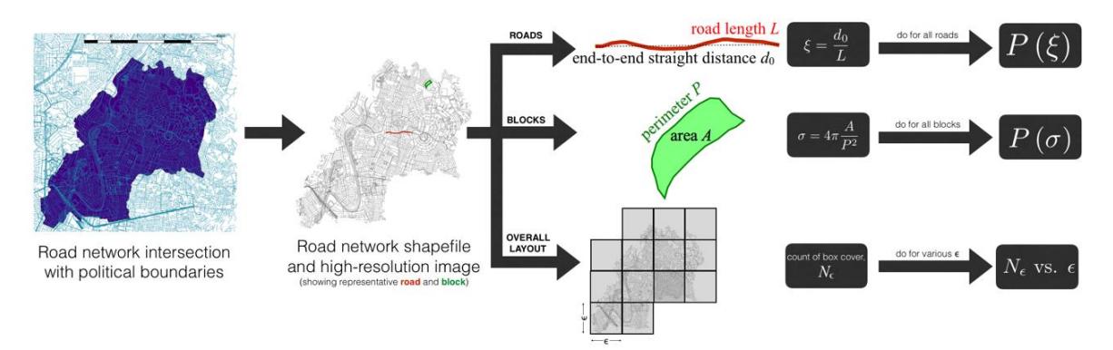
Figure 3. Flow of the procedure for characterization (here, the representative city is Marikina, Metro Manila). (Left to right) From the road network obtained in OSM, the political boundaries of the city are used to get the collection of roads and blocks to be analyzed. For each road, the straightness \(\xi\) is computed; for each block, the circularity \(\sigma\) is computed; and for the entire road network layout, the number of \(\epsilon \times \epsilon\) boxes used to fill the entire pattern, \(N_{\epsilon}\), is counted. Doing the procedure for all roads, blocks, and box sizes, respectively, results in the statistical characterization.
To get the dimensionless shape metrics, the individual roads r and blocks b are obtained from the GIS data. The node-to-node distances \(\ell\) are computed from the coordinates \((\phi_r, \theta_r)\) using the great-circle distance formula,
\[\ell = R_E \arctan \left[ \frac{\sqrt{(\cos \theta_2 \sin \Delta \phi)^2 + (\cos \theta_1 \sin \theta_2 - \cos \theta_2 \sin \theta_1 \cos \Delta \phi)^2}}{\sin \theta_1 \sin \theta_2 + \cos \theta_1 \cos \theta_2 \cos \Delta \phi} \right]\] (5)
where a spherical Earth assumption with radius \(R_E \approx 6371\) km is used, and \(\Delta \phi = |\phi_2 - \phi_1|\). The assumption of a spherical Earth introduces inherent errors, but these are deemed to be small enough considering the relatively small geographical windows involved. Additionally, the computations done using Eq. (5) do not account for elevation. The planar length of the road is thus \(L_r = \sum_r \ell_r\), which is deemed to be sufficiently accurate for our purpose. The straight end-to-end distance \(d_0\), on the other hand, can be computed from Eq. (5), with \((\phi_1, \theta_1)\) and \((\phi_2, \theta_2)\) being the start and end points of r, respectively. The set of all computed straightnesses, \(\xi = \{\xi_r\}\), is then collected for statistical analyses.
For each city, the road networks and the political boundaries are also drawn as maps with street traces and stored as raster images with a minimum of 1:20,000 scaling. When stored under a resolution of 600 dpi, each pixel corresponds to \(0.85 \times 0.85\) m patches of actual area, deemed to be accurate enough to account for the actual morphologies on the ground. The images were processed in MATLAB for morphological feature extraction. The image of every city and municipality was processed for the area \(A_b\) and the perimeters \(P_b\) of road bounded blocks b, here measured in pixels. The circularities were straightforwardly computed from Eq. (2) and stored as the set \(\sigma = \{\sigma_b\}\) for statistical analyses.
Finally, to obtain the box-counting dimension \(\delta\), we used box sizes \(\epsilon\) measured in pixel units and plotted the \(N_{\epsilon}\) versus \(\epsilon\) plot. We used the discrete power-law fitting by Alstott et al. (2014) based on the Kolmogorov-Smirnoff condition (Clauset et al., 2009) to determine the best-fit exponent for the decaying power-law.
Results
Qualitative descriptions and morphological characterization
In Figure 4, the road network layouts of the key cities in the conurbations are presented. One readily notices the key differences in the network architectures due to the different geographical factors. Consider first the conditions for the Metro Manila conurbation and the City of Manila, in particular. The metropolitan region as a whole has the smallest area among the conurbations in Table 1, and is situated in an isthmus, constrained on the west by the Manila Bay and the Laguna Lake, respectively. The City of Manila itself is bounded on the west by the Manila Bay and the Pasig River cuts through the middle portion of the city. Despite this, the NCR has been the main recipient of the economic growth of the country, which has increased in pace over the last few years (World Bank 2015). These conditions resulted in a densified road configuration, wherein the available area has been subdivided into homogenized blocks by the creation of grid-like roads (Strano et al., 2012). As a result, the road network of Manila is dominated by grid formations, which is evident from the snapshots shown in Figure 4(a).
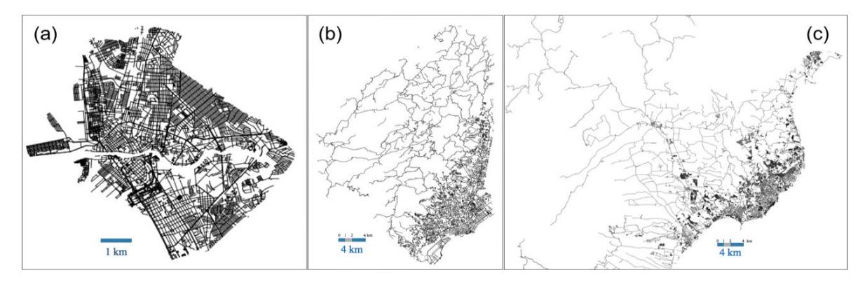
Figure 4. Road network layouts: representative cities. (a) The constrained location of Manila, along with the fast-paced economic growth, led to the formation of a highly densified grid networks. (b) The city of Cebu has densified formations at the eastern section and sinuous roads towards the mountainous regions in the east. (c) Davao City (not the whole area is shown; only a portion with comparable scaling) is the largest Philippine city in terms of geographical area, and, similar to Cebu, dense urban grids can be found at the eastern portion near the port area.
The Metro Cebu and Metro Davao conurbations are relatively bigger than Metro Manila in terms of land area. Similar to Manila, the cities of Cebu and Davao are also port cities, bounded by water at their eastern portions. However, both Cebu and Davao are bounded by mountainous regions on their north and western sides. In Figure 4(b) and (c), we can see that the grid-like formations of the urban landscape are only apparent near the east coasts of Cebu and Davao, while their western portions are dominated by sinuous mountain roads and trails.
The road network layouts of the representative cities support the observations of Strano et al. (2012) regarding the simple rules obeyed by road network growth. As noted earlier, exploration is succeeded by homogenization, resulting in densification of the core urban area (Strano et al., 2012). Despite the common forcing mechanisms, however, Figure 4 illustrates that the resulting spatial layouts vary significantly, due to differences in the extent of exploration and densification among the cities investigated. These differences, in turn, are ultimately due to the age, socioeconomic conditions, and geographical constraints experienced by the cities.
To provide a quantitative characterization for the observed qualitative differences, we obtained the statistical distributions of the dimensionless shape parameters. In Figure 5, the distributions of the straightnesses, (), and circularities, (), are plotted on the left and right panels, respectively. To highlight the differences, the cities from the same metropolitan conurbations were plotted together, and the conurbations were separated into the different rows.
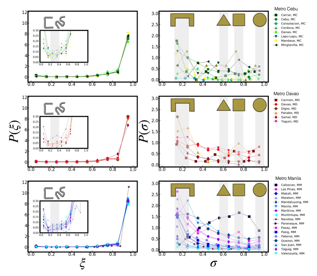
Figure 5. Distributions of the dimensionless shape parameters [left panels: straightness distributions; right panels: circularity distributions; rows: conurbations; scales are preserved]. Left panels: The straightness distributions are dominated by ξ = 1 (straight roads). Left panel insets: When zoomed in, a characteristic peak is observed near ξ = 0.3 [shaded regions]. These values are due to commonly appearing road motifs: (i) minor roads that start and end from a main road and create a C-shaped path with equal three equal segments, resulting in ξ = 1/3; or (ii) highly sinuous roads that follow the terrain, with ξ →1/π. Right panels: The circularity distributions peak at small values due to concave irregular shapes and at larger values correspond to regular polygons. As a guide to the eye, representative shapes and their range of values are shown [shaded regions].
Because roads are created to connect two important points in space, there should be a preponderance of straight roads. Therefore, in the left panels of Figure 5, we find that the straightness distributions for all metropolitan regions all have sharp peaks at = 1. To observe the finer details of the distribution, we plot in the inset the same () but now focusing on the smaller straightness values. The peak near = 0 is due to closed loops of roads such as rotundas, which are also present in the urban road network architecture. We also highlight an interesting region in the () distribution, shown in the shaded regions near the left panel insets. Here, we find that there is a slight peak around the value ≈ 0.3. These peaks are deemed to result from two types of road network motifs, whose relative shapes are illustrated as guides to the eye on top of the shaded regions.
The first common motif is mostly found in grid-like urbanized regions. In some cases, blocks are formed beside a main road by creating a minor road that follows the sides of a rectangle. The main road itself forms one of the sides, while the minor road traverses the three other sides. This forms a C-shaped road, as illustrated in the left-panel insets; note that, in very regular square grids, this road shape will have straightness values of exactly = 1/3, thus contributing to the statistics at this value. The other contributing motif is more likely to be found in portions with the dominance of exploratory roads. In a previous work, Cirunay & Batac (2021) observed minor peaks in the straightness distribution for = 1/. This value of the straightness corresponds to the case of roads following the natural landform; it has been shown that rivers and other natural linear formations approach a sinuosity (inverse of straightness) of π due to self-organization (Stølum, 1996). In the insets of the left panels of Figure 5, an illustration of such a highly sinuous road that conforms to the geography is also presented on top of the shaded region. Despite the differences in the visual patterns of the road networks, the three metropolitan regions all show significant statistics at the shaded characteristic value due to these expected shapes, both in densified and exploratory regimes.
The morphological descriptions of the blocks are presented in the right panels of Figure 5, which shows the distributions of the circularities of the city blocks, (), for the three conurbations. We removed the very small thin shapes with → 0 because they are incidental in nature and are mostly due to small strips of area segmented within inner city roads and at the boundaries. Despite the removal of these shapes in the statistical description, we find increased incidence of circularities at around ≈ 0.2, shown as the leftmost shaded regions. Upon closer inspection, these values are found to be due to concave regions bounded by concentric C-shaped minor roads emanating from a common main road. A representative concave shape is illustrated at the top of the shaded region. Incidentally, for a very simple case of rectangular concentric roads, simple geometric analyses reveal the common origins of these characteristic values of circularities of the block and their corresponding straightnesses of the concentric roads bounding it.
The other shaded regions in the right panel of Figure 5 correspond to regular geometric shapes of blocks. From the definition of the circularity given in Eq. (2), the values for the regular shapes are shaded in the right panels of Figure 5: for a triangle, = √3⁄9 ≈ 0.61; for a square, = /4 ≈ 0.785; and for a perfect circle, = 1. As expected, all conurbations show peaks near the circularity of the square due to the densified grid portions in their urbanized zones.
The distributions () and () in Figure 5 therefore give complementary descriptions of the road network morphology that are consistent with the qualitative observations from the map layouts presented in Figure 4. These purely spatial and morphological descriptions highlight the fact that no two cities are created equally; the complex interrelationships between geographical, socio-economic, political, and even cultural differences among the cities play important roles in the resulting subdivision of the available space by the road network layouts. Despite the differences, however, we observe general trends in the resulting distributions, especially the emergence of key values that dominate the cities' morphological features. These values, as highlighted in Figure 5, are brought about by the repeating road network motifs that are expected to be found across these cities regardless of their history and geography. We can therefore think of the spatial characterization by morphological feature statistics as a quantitative method to reveal the commonalities among cities.
Fractal dimensions of component cities
The plot of the box counts versus box dimension for the component cities and municipalities of the three metropolitan regions of the Philippines is plotted in Figure 6 below. The conurbations are separated in the different panels for clarity. For each metropolitan region, the dashed lines corresponding to the minimum and maximum scaling exponent among the component cities are presented as guides to the eye.
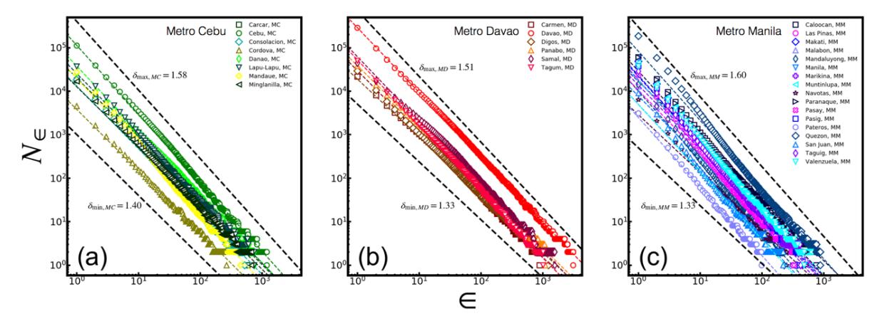
Figure 6. Box-counting dimensions [panels: metropolitan regions; symbols: data; colored dashed lines: power-law fits; black dashed lines: limiting fractal dimensions per conurbation, shown as guides to the eye]. The (a) Metro Cebu, (b) Metro Davao, and (c) Metro Manila conurbations all show power-law versus plots spanning almost three orders of magnitude. The statistical best fits ~ − revealed power-law exponents within the range ∈ [1.33, 1.60).
The box counts data from Figure 6 [colored symbols] were statistically analyzed using the powerlaw Python package (Alstott et al., 2014, Clauset et al., 2009) to obtain the best exponent of the power-law trend ~ − . All the computed fractal dimensions of the street network layouts of the cities and municipalities were found to be between linear and planar dimensions, with the smallest exponent = 1.329 obtained for Digos City in Metro Davao and the highest exponent = 1.605 for Mandaluyong City in Metro Manila. Incidentally, the obtained fractal dimensions for every city did not show strong correlations with other city properties such as size, population, and assets. Figure 7 presents all cities and municipalities from all the conurbations as single points, whose x-components are the fractal dimensions and the y-components are the other spatio-economic properties.
The very weak correlation of fractal dimension with the other properties of the city is a notable result. In previous works, several authors have noted that city properties show universal scaling behavior with population; that is, when the data about a property (e.g., average income, number of patents, and even crime incidence) is collected for all cities in a country or a region, the scattergrams of values versus the corresponding population of the city will show a powerlaw behavior, ~ (Bettencourt et al., 2007; Bettencourt, 2013). Although other works have shown the limitations of this behavior (Arcaute et al., 2015; Depersin & Barthelemy, 2018), it has
become so useful that by only looking at the population of a city a good approximation for its property can already be inferred (Bettencourt et al., 2007; Lobo et al., 2013). Incidentally, one class of properties that appear to scale with city population are infrastructure related properties, with a sublinear scaling exponent ≈ 0.8 < 1. One such property is the road network cover (Bettencourt et al., 2007). In a previous work on Philippine cities, the scaling behavior of total city road length with population was observed but with a different exponent from the ones observed for other countries (Cirunay & Batac, 2018b), most likely due to data sparsity (Depersin & Barthelemy, 2018). It should be noted, however, that the fractal dimension is not one of the infrastructure-related properties that are reported to scale with city population.
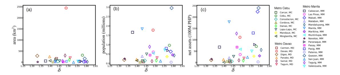
Figure 7. Scattergrams of city properties with fractal dimensions with (a) area; (b) population; and (c) net assets (COA 2019). There is no statistically significant correlation between any of these city properties with fractal dimension.
The fractal dimension, therefore, can be thought of as a quantitative measure of a city road network's unique 'fingerprint', one that incorporates all of the conditions experienced by the individual urban area throughout its historical development that led to the current road network architecture. Unlike other city properties, which have been described by scaling arguments in previous works, the fractal dimension cannot be simply inferred from its correlation with other city metrics. In fact, even cities with very similar geographies and socio-economic conditions may manifest vastly different fractal dimensions. Similar to the statistical distributions of morphological metrics, the fractal dimension is a spatial characterization; unlike these shape factors, however, the fractal dimension encapsulates the differences instead of the commonalities between cities.
Discussions and Implications
The results validate the complex nature of road network formation in the form of the observed commonalities in the statistical distributions of the morphological metrics shown in Figure 5. The mechanisms of road growth in all the metropolitan conurbations of the Philippines show similar characteristics due to the common mechanisms of exploratory and densified road network growth (Strano et al., 2012). In self-organized urban conditions, the way a road winds through and divides the space is driven by the same mechanisms that aim to straightforwardly connect two regions, with the goal of minimizing the cost and, ideally, travel time. Incidentally, such simple local mechanisms, when viewed from a collective perspective, prove counterproductive and even end up degrading the overall flow in the network.
As such, the observed differences deserve more immediate attention due to their implications for the actual conditions on the ground. The differences in geography give rise to differences in road network layout and density, as can be seen from the snapshots of the key cities in Figure 4. In particular, the capital region centered in Manila has been reported to have undergone rapid road network growth over just the last three decades (Cirunay et al., 2020), resulting in the most
congested road network in developing Asia (ADB 2019), affecting the thirteen million inhabitants of the densest megacity in the world (United Nations DESA 2019). On the other hand, while Metro Cebu and Metro Davao may still continue exploration at the mountainous regions, and thus may densify to have more homogeneous fractal dimensions (Murcio et al., 2015), the regions that are already densified may face the same constriction and related challenges over the next few decades.
Conclusion
We have shown a straightforward way to quantitatively describe the complexity of road networks through two characterization procedures that highlight different aspects of road architecture comparisons. On the one hand, by collecting all morphological shapes created by the layout of individual streets, we have presented the distributions of the dimensionless metrics straightnesses (of individual roads) and circularities (of individual blocks). On the other hand, the entire road layout was also characterized by the unified fractal dimension using the box-counting technique. When applied to representative cities and municipalities belonging to the major economic centers of the Philippines, the former revealed the commonalities between the cities in the form of recurring network motifs, while the latter quantified the differences in the form of a unique fractal dimension that is not in any way correlated with other city characteristics.
Road networks are framed from a complex systems perspective, and this work has highlighted the emergence of complexity in the urban geographical layout. Local rules on the ground, along with conditions dictated by geography, economy, and policy were shown to give rise to stark visual differences in the resulting architectures. The presented methodologies to quantify these patterns are deemed to be straightforward enough to be extended to other city road networks. In fact, for morphological characterization, previous works have suggested that the common motifs found in the city data sets in the respective works were also present in other cities in other regions of the world (Lämmer et al., 2006; Masucci et al., 2013), even though measured using equivalent but slightly different metrics (Bribiesca, 2008). The measured fractal dimensions, which have been found not to follow simple scaling relations with population and other factors, provide a simple quantitative measure, one that incorporates the various local factors present in the development of the individual roads in their respective regions. We believe that the method used in this work should be applied to other urban centers in the world, especially those from the global south, where there is an expected faster pace of growth over the next few decades (United Nations DESA 2019).
This work presents an important addition to the scientific literature by focusing on geographically and socio-economically disparate urban centers in an archipelagic setting. Most of the previous spatial characterization works have been done on large continental settings for cities in countries from the global north (Lämmer et al., 2006; Masucci et al., 2009; Courtat et al., 2011; Barthelemy et al., 2013). Characterizing Metro Manila (Cirunay & Batac, 2018) along with Metro Cebu and Metro Davao provides an important benchmark for comparing road networks originating from different islands within the same country. As expected, these metrics may continue to change as these urban regions mature (Murcio et al., 2015), so more work needs to be done to continue the characterization. With the additional analyses using more accurate and recent data sets, a better quantitative historical description of these cities can be made (Cirunay et al., 2020), which can lead to the identification of further regions of growth (Xu et al., 2015). This, in turn, can be used for better management of these urban metropolitan regions and may pave the way for policy decisions that will lead to further sustainable growth.
Acknowledgments
M.T.C. acknowledges the financial support from the Department of Science and Technology (DOST) Science Education Institute (SEI) through the Advanced Science and Technology Human Resources Development Program (ASTHRDP) scholarship.