Regional Variations of Indonesian Cities: Geometric properties, Street Patterns, and Topological structure.

Muhammad Fajri Romdhoni; Mahbub Rashid

doi:10.5614/jpwk.2022.33.3.2

Regional Variations of Indonesian Cities: Geometric properties, Street Patterns, and Topological structure.

Published: 2022-12-23 | DOI: 10.5614/jpwk.2022.33.3.2 | Vol 33, Issue 3 (2023) | Cited by: 1

Authors

Muhammad Fajri Romdhoni

Universitas Sriwijaya, Jl. Raya Palembang - Prabumulih Km. 32 Indralaya, OI, Sumatera Selatan 30662

ORCID: 0000-0002-3145-940X · OpenAlex: A5069180852

Mahbub Rashid

School of Architecture and Design, University of Kansas

OpenAlex: A5114028107

Abstract

As one of the fastest growing countries with the largest population in the ASEAN region, cities in Indonesia are constantly evolving and changing. Although the current political establishment is planning to relocate the country’s capital to the Kalimantan island, comparative research on Indonesian cities is very limited. Indonesia is an archipelago country that consists of 17,508 islands and at least 514 urban areas, of which 98 of them can be categorized as cities. This paper will focus on examining variations in provincial capital cities from Indonesia’s 6 regions: Sumatera, Java-Bali, Nusa Tenggara, Kalimantan, Sulawesi, Maluku-Papua. The paper uses OpenStreetMap (OSM) vector datasets to study the geometric properties of street centerlines and the regression techniques on the Landsat satellite images of these cities processed in GIS to study land-use patterns. The paper also uses the method of patterns classification from volunteered geographic information systems (VGI) to study street orientational patterns utilizing OSMnx. Finally, the paper uses space syntax methods to describe the topological features of natural street networks of the cities. The results of this study show that there are statistically significant regional variations among cities in Indonesia. They also show that street network orientations are correlated with global integration values indicating that movement potentials could be affected by spatial shape patterns in these cities.

Keywords

Geography; Indonesian; Regional science; Economic geography; Population; Cartography; Demography; Sociology

1. Introduction

According to World Cities, a United Nations report on global urbanization trends(United Nations, 2018), in 2018, the world's fastest-growing cities were in Asia and Africa. According to the same report, cities with 500,000 inhabitants or more will grow at an average annual rate of 2.4 percent to 6 percent in these regions. At least fourteen cities with more than one million people are located in Indonesia, stated the report. More cities with one million or more inhabitants will certainly emerge in the country. Indonesian society has been predominantly urban since 2012 (Jones & Mulyana, 2015). By 2045, 220 million people will live in urban areas (Roberts et al., 2019). While the country is rapidly developing, there is a lack of comparative quantitative studies on urban geometries and street networks to help us better understand the cities of the country.

This study used six main regional groups of islands in Indonesia, i.e., Sumatra, Java-Bali, Nusa Tenggara, Kalimantan, Sulawesi, and Maluku-Papua (Figure 1). Dramatic differences in population distribution among these regions have significantly affected the trends of Indonesian city development. The Java-Bali region is the most populated in Indonesia with 56.7 percent of the country's 270.63 million people. The very high concentration of urban developments on Java and the overburdening of Jakarta as the nation's capital are among the reasons why the country plans to move its capital to a more 'neutral', less developed region. This is not surprising, since other neighboring nations have successfully relocated their old capitals to new places, such as from Melbourne to Canberra in Australia, Kyoto to Tokyo in Japan, and from Kuala Lumpur to Putrajaya in Malaysia.

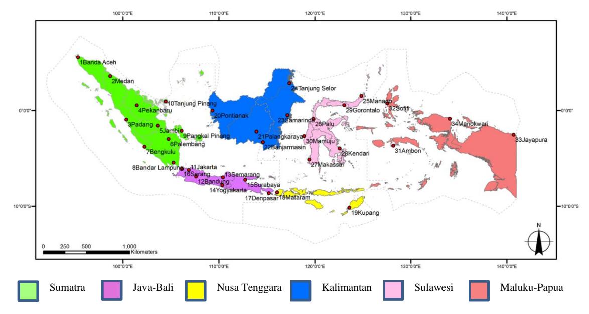
Figure 1. Regional map of Indonesia and 34 provincial capitals as case study cities. Source: Author 2021

It is difficult to study Indonesian cities due to their differences in geographical, historical, and social contexts. The layouts of many Indonesian cities were historically influenced by colonialism from the sixteenth to the nineteenth centuries (Ford, 1993). Many early cities were also influenced by their geographical site, as many of them have a coastal setting or rivers that cut through them. Additionally, some inland cities take advantage of natural aesthetics. Then there are those that were built to serve industrial or governmental needs.

There is a pressing need to study the geometry of Indonesian cities because these cities have undergone significant morphological changes since the Dutch colonial period, which started in the seventeenth century. Studies involving colonial cities in non-European countries have shown that colonization generally had a significant influence on the spatial configuration and geographical model of cities. According to these studies, European mercantile cities were modified in the colonies to accommodate the local inhabitants while providing colonial settlements and military cantonments in the outer zones of the city (Kosambi & Brush, 1988). Therefore, the configuration of most colonial port cities in South Asia had a strong resemblance to that of European mercantile cities with adaptations to geographical features and military needs (Bowden, 1972; Hornsby, 1997) (see Figure 2). Indonesian colonial cities may have followed the same transformation patterns. First, European-style aesthetic features were imposed. Later, Indonesia's cultural and geographical environments were adapted to fit these features.

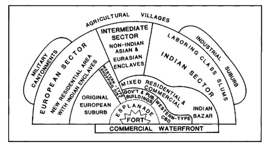
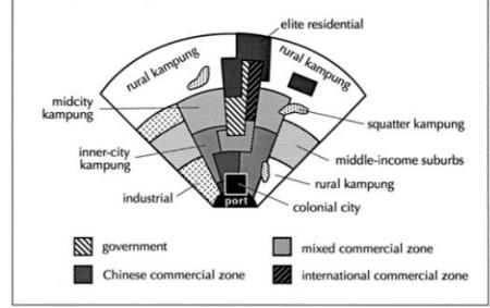
Figure 2. Classical model of Southeast Asian cities. Left: Schematic of a colonial port city. Right: Model of the topographic structure of an Indonesian city. Source: M. Kosambi and J.E. Brush (1998) and Ford (1993)

After Indonesia's independence, political leaders of the country embraced modern urban ideologies. Indonesia's first president Sukarno wanted to unite Indonesia by promoting the image of the country as a rising power in the developing world and by distancing the nation's image from its colonial heritage (Ford, 1993). In A Model of Indonesian City Structure, Ford explained that many national-scale urban projects were carried out during this time. Yet, the lack of connections among the islands of the Indonesian archipelago resulted in different patterns of urban development in different regions. It is generally assumed that the differences between Indonesian cities grow as the distance between a region and the central territories increases in term of social, economic, and urban development patterns.

No previous study has verified this assumption, further indicating the need for more study on the morphology of Indonesian cities, which is also indicated by the fact that existing morphological studies on Indonesian cities did not systematically compare their differences. One of these existing studies looked at the relationship between location and the historical morphology of Southeast Asian coastal cities, including some from Indonesia, using historic morphological analysis (Widodo, 2004). Another study compared the visual morphology of some cities on Java island (Sunaryo et al., 2012). Yet another study showed that there are significant similarities

between three Indonesian cities and Amsterdam and Delft (Tutuko et al., 2018). Most systematic comparative studies on cities have been conducted in North America, Europe (Kruger, 1989; Law et al., 2012; Oliveira et al., 2015; Siksna, 1998) and China and Japan in Asia (X. Chen, 2018; X. F. Chen, 2018; Park et al., 2014; Sun, 2013). In one example, a broad comparison of cities was done by Rashid (2017), who studied the topological properties, angular, and rank-size distribution metrics from axial and segment maps of two-square-mile urban layouts of more than a hundred large cities in different countries around the world. Another study that compared street network patterns based on grid entropy and street network orientation was done by Boeing (Boeing, 2019). Similar comparative studies do not exist for Indonesian cities.

Jakarta – West Indonesia (11) Samarinda – Central Indonesia (23) Jayapura – East Indonesia (33)

Figure 3. Pattern and density differences between Indonesian cities. Source: Author, 2020; extracted from OpenStreetMap, OSMnx compiled using ArcGIS 10.4.

2. Materials and Methods

The main purpose of this study was to classify regional variation in the morphology of Indonesian cities. This study had three objectives. The first objective was to understand the geometric properties and geometric densities of Indonesian cities. The second objective was to understand street network patterns using grid entropy. The third objective was to compare cities using the space syntax method to understand their topological structure. We looked at the distribution patterns of the global integration values of the axial segments in axial maps of the cities. These three urban characteristics in six different main regions (Sumatra, Java-Bali, Nusa Tenggara, Kalimantan, Sulawesi, Maluku-Papua) were compared to understand the regional variations. The significance level of the differences between cities from different regions were determined using one-way ANOVA (Field, 2007). Linear regression analysis was used to explore if there were any statistically significant relationships between the categories.

2.1. Case studies

For this comparative study, 34 provincial capitals in Indonesia were chosen (Figure 1 and Table 1). They included a wide range of Indonesian cities, with different sizes and economic characteristics (large metropolitan, metropolitan, non-metropolitan urban areas), geographical locations (coastal, river, and inland), and population densities. It is worth mentioning that several highly populated metropolitan cities in Indonesia were not taken as case study cities in this research, including Bogor, Malang, Surakarta, and Sukabumi, because they do not serve as provincial capital.

The case study cities were selected from six main regions of the country. They consisted of ten cities from Sumatra; seven cities from Java & Bali; two cities from Nusa Tenggara; five cities from Kalimantan; six cities from Sulawesi; and four cities from Maluku & Papua. The case study cities were also divided into coastal, river, and inland cities based on their locations.

2.2. Methods of Analysis

The research used geometrical measures such as total street length, mean street length, total number of street segments, built-up area density, city administrative size, and linear density. The total street length was used to describe the total number of street lines, based on which the area coverage of the street network in the study area could be determined. The mean street length was determined by dividing the street's total length with the total number of street centerlines. The street's mean length describes the average street length, hence describing the overall average value of the distance between the street centerline and the length between blocks in the study area. The street's maximum length describes the longest street centerline in each case study and indicates the length from the respective points. The total number of street segments describes the total number of streets in the case study. Linear density is a measurement of the total street length weighted by administrative size.

Table 1. The 34 case study cities of Indonesian provincial capitals.

No.	Name	Regional	Administrative	Population	Population	Density	Location
		group	area km²	2016	density/km²	•
1	Banda Aceh		61.36	254,904	4,552	Н	Coastal
2	Medan		265.10	2,229,408	8,409	H	Inland/C
3	Padang		694.93	914,968	1c,316	M	Coastal
4	Pekanbaru		632.26	1,064,566	1,638	M	Inland/R
5	Jambi		205.58	583,487	2,838	M	River
6	Palembang	(1)	400.61	1,602,071	3,999	H	River
7	Bengkulu	Sumatra	151.70	359,488	2,369	M	Coastal
8	Bandar	Sumana	197.22	997,782	5,058	H
	Lampung						Coastal
9	Pangkal		118.41	204,735	1,720	M
	Pinang						Coastal
10	Tanjung		150.86	204,735	855	L
	Pinang						Coastal
11	Jakarta		662.33	10,177,924	15,366	H	Coastal
12	Bandung		167.31	2,490,622	14,886	H	Inland
13	Semarang	(2)	373.70	1,602,717	4,289	H	Coastal
14	Yogyakarta	Java-Bali	32.50	417,744	12,853	H	Inland
15	Surabaya	Java-Dan	326.81	2,862,406	8,758	H	Coastal
16	Serang		266.74	643,205	2,412	M	Inland/C
17	Denpasar		127.78	897,300	7,022	Н	Coastal
18	Mataram	(3) Nusa	61.30	459,314	7,493	Н	Coastal
19	Kupang	Tenggara	180.27	402,286	2,232	M	Coastal
20	Pontianak		107.82	618,388	5,736	Н	River
21	Palangkaraya	(4)	2,678.51	331,115	112	L	River
22	Banjarmasin	Kalimantan	98.46	684,183	9,414	H	River
23	Samarinda		718.00	812,597	1,132	M	River

24	Tanjung		677.77	49,242	72	L
	Selor						River
25	Manado		157.26	417,906	2,721	M	Coastal
26	Palu		395.06	374,020	946	L	Coastal
27	Makassar	(5)	175.77	1,469,601	8,360	Н	Coastal
28	Kendari	Sulawesi	295.89	359,371	1,215	M	Coastal
29	Gorontalo		65.96	195,468	2,963	M	Coastal
30	Mamuju		5,064.19	138,698	54	L	Coastal
31	Ambon*	(6)	359.45	427,934	1,190	M	Coastal
32	Sofifi	(6) Maluku -	20.98	1,783	84	L	Coastal
33	Jayapura		940.00	288,786	307	L	Coastal
34	Manokwari	Papua	3,186.28	162,578	51	L	Coastal

Urban density analysis using land use—land cover (LULC) classification and population density analysis were performed using remote sensing analysis in ArcMap. Band regression calculation and pixel learning techniques were used to compare the LULC of the case study cities (Joseph et al., 2012; Li & Weng, 2005; Romdhoni, 2020). The generated pixels were used to verify urban built-up areas. The built-up area density shows the weighted built-up land cover of the case study cities.

For the space syntax analysis, we used street centerline maps of 30 x 30 km, or 900 km<sup>2</sup>, of each of the 34 cities. These maps were converted to a GIS-based platform using Shapefile for ArcGIS. ArcGIS 10.4 was applied, using Axwoman 6.3 for axial and natural street data conversion (Jiang, 2015, 2019). The street centerline segment maps were then digitized from space syntax natural street to axial line using the Axwoman plugin tool in ArcGIS for further syntax analysis, such as global integration, local integration, connectivity, and choice. The space syntax measurement was then used to define the foreground and background patterns proposed by Hillier (2016).

2.3. OpenStreetMap and OSMnx

OpenStreetMap (OSM) is a useful resource for up-to-date and actual vector street maps of cities around the world. It is a collaborative mapping project that supplies free, editable maps. OSM is one of the most successful volunteered geographic information (VGI) projects (Fan et al., 2014). OSM originally imported the 2005 TIGER/Line (Topologically Integrated Geographic Encoding and Referencing system of the US Census Bureau) (Zielstra et al., 2013). Since then, there have been corrections and improvements on the OSM open-source data. Research has shown that the map accuracy and data quality are relatively high (Barron et al., 2014; Girres & Touya, 2010; Haklay, 2010), also for cities in developing countries (Minaei, 2020). OSMnx was developed by Boeing (Boeing, 2017) to analyze the topological information of geometric data collected from OSM. This research used OSMnx for its purpose.

Figure 4. OSMnx provides not only a visual representation of formal/grid patterns or natural/organic patterns, but also topological configuration analytics. Source: Boeing, 2019

2.4. Quantifying Order, Disorder, and Correlations

Shannon entropy (Shannon, 1948) was used to understand and quantify the formal or natural order of the street networks. Boeing (Boeing, 2019) incorporated Shannon entropy into the OSMnx software to calculate the bearing angle of every edge (i.e., the orientation of every street) of a street network. The street orientation information is stored in 36 equal-sized bins representing 360 degrees. Entropy suggests that the street network orientation is 'fully grid' if the value is 1 and 'natural/organic' with multiple street angularities if the value is closer to 0.1 (Boeing, 2019).

2.5. Space Syntax Methods and Measurements

Space syntax was initially proposed in the 1970s as an approach to study the morphology of cities (Hillier et al., 1976). Its theories and methods can reveal the role of spatial configurations in shaping different social phenomena and urban forms (Hillier, 2005, 2008; Hillier & Hanson, 1989; Hillier & Iida, 2005; Peponis et al., 1989; Rashid & Shateh, 2012). Space syntax distinguishes itself from other morphological methods using quantitative methods and measurements (Rashid, 2019). Space syntax analysis has evolved from the original axial analysis method, which can be interpreted as shifting from street-like elements (Turner et al., 2005) to segment analysis (Turner, 2007). Axial line and axial segment are topological models that use lines to represent spaces in urban environments. Axial lines are straight lines of movement and visibility using the minimal set of axial lines. In comparison, segments are parts of the axial lines broken at the intersection points with other axial lines (Rashid, 2019). The configuration of lines from axial and segment maps allows the researcher to analyze the pattern relation based on syntactic values or graph theory using assigned color ranges.

The space syntax method produces measurements such as integration, choice, and intelligibility, to describe and evaluate spatial configurations. Integration in space syntax indicates the value of accessibility or how well connected an axial line is with the other axial lines in an axial map. A high integration value, traditionally represented with the color red, indicates that the line is better connected as opposed to a low integration with fewer connections, for which usually the color blue is used. Integration is a measure of syntactical accessibility; a high integration value is an indication of high density and movement in urban areas (Hillier, 2007; Hillier & Hanson, 1984). This study used these integration measurements to reveal hierarchical network patterns in the spatial layouts of the Indonesian cities.

The measurements and methods of space syntax have significantly affected urban morphological studies. They help explain how cities work. Hillier (2012b, 2012a, 2016) proposed the idea of the generic city composed of two inter-related networks. The foreground network is made up of a small number of longer axial lines with route continuity (Turner, 2007), while the background network consist of a larger number of shorter lines that emphasize local interactions. The foreground network is the 'city-making process', concentrating on maximizing movement, making it suitable for microeconomic activities. In contrast, the background network provides a diffuse movement structure, defining residential processes.

3. Results

3.1. Indonesian Cities Geometry

The first findings of this research were the geometric properties of the Indonesian case study cities. From the 34 provincial capitals, we gathered information on their geometrical properties, i.e., total street length, mean street length, maximum length of street, total number of street segments, which are shown in Table 2. This table also shows the linear density and built-up area density of these cities.

Table 2. Geometric properties of 34 Indonesian provincial capitals according to regional classification.

1 Banda Aceh 880,984 76.81 3,122 11,469 0.13 14.36 2 Medan 4,160,857 72.1 7,292 57,704 0.14 15.70 3 Padang 2,168,739 76.52 3,925 28,342 0.05 3.12 4 Pekanbaru 4,071,861 82.66 4,683 49,256 0.17 6.44 5 Jambi (1) 1,608,264 80.99 4,008 19,857 0.08 7.82 6 Palembang Sumatra 2,155,230 113.18 6,004 56,117 0.29 5.38 7 Bengkulu 1,143,667 76.86 2,958 14,879 0.08 7.54 8 Bandar Lampung 2,055,671 74.69 2,757 27,522 0.11 10.42 9 Pangkal Pinang 591,610 109.92 4,208 5,382 0.14 5.00 10 Tanjung Pinang 510,541 131.37 4,384 3,886 0.16 3.38 11 Jakarta 12,533,903 73.1	No.	Name	Regional group	Total street length (m)	Mean street length (m)	Maximum street length (m)	Total number of street segments	Built- up area density	Linear Density
3 Padang 2,168,739 76.52 3,925 28,342 0.05 3.12 4 Pekanbaru 4,071,861 82.66 4,683 49,256 0.17 6.44 5 Jambi (1) 1,608,264 80.99 4,008 19,857 0.08 7.82 6 Palembang 2,155,230 113.18 6,004 56,117 0.29 5.38 7 Bengkulu 1,143,667 76.86 2,958 14,879 0.08 7.54 8 Bandar Lampung 2,055,671 74.69 2,757 27,522 0.11 10.42 9 Pangkal Pinang 591,610 109.92 4,208 5,382 0.14 5.00 10 Tanjung Pinang 510,541 131.37 4,384 3,886 0.16 3.38 11 Jakarta 12,533,903 73.13 6,908 171,379 0.46 18.92 12 Bandung 2,949,956 69.81 8,007 42,253	1	Banda Aceh		880,984	76.81	3,122	11,469	0.13	14.36
4 Pekanbaru 4,071,861 82.66 4,683 49,256 0.17 6.44 5 Jambi (1) 1,608,264 80.99 4,008 19,857 0.08 7.82 6 Palembang 2,155,230 113.18 6,004 56,117 0.29 5.38 7 Bengkulu 1,143,667 76.86 2,958 14,879 0.08 7.54 8 Bandar Lampung 2,055,671 74.69 2,757 27,522 0.11 10.42 9 Pangkal Pinang 591,610 109.92 4,208 5,382 0.14 5.00 10 Tanjung Pinang 510,541 131.37 4,384 3,886 0.16 3.38 11 Jakarta 12,533,903 73.13 6,908 171,379 0.46 18.92 12 Bandung 2,949,956 69.81 8,007 42,253 0.14 17.63 13 Semarang 4,193,545 72.24 8,041 58,045	2	Medan		4,160,857	72.1	7,292	57,704	0.14	15.70
5 Jambi (1) 1,608,264 80.99 4,008 19,857 0.08 7.82 6 Palembang 2,155,230 113.18 6,004 56,117 0.29 5.38 7 Bengkulu 1,143,667 76.86 2,958 14,879 0.08 7.54 8 Bandar Lampung 2,055,671 74.69 2,757 27,522 0.11 10.42 9 Pangkal Pinang 591,610 109.92 4,208 5,382 0.14 5.00 10 Tanjung Pinang 510,541 131.37 4,384 3,886 0.16 3.38 11 Jakarta 12,533,903 73.13 6,908 171,379 0.46 18.92 12 Bandung 2,949,956 69.81 8,007 42,253 0.14 17.63 13 Semarang 4,193,545 72.24 8,041 58,045 0.31 11.22 14 Yogyakarta Java-Bali 569,330 84.2 2,099	3	Padang		2,168,739	76.52	3,925	28,342	0.05	3.12
6 Palembang Sumatra 2,155,230 113.18 6,004 56,117 0.29 5.38 7 Bengkulu 1,143,667 76.86 2,958 14,879 0.08 7.54 8 Bandar Lampung 2,055,671 74.69 2,757 27,522 0.11 10.42 9 Pangkal Pinang 591,610 109.92 4,208 5,382 0.14 5.00 10 Tanjung Pinang 510,541 131.37 4,384 3,886 0.16 3.38 11 Jakarta 12,533,903 73.13 6,908 171,379 0.46 18.92 12 Bandung 2,949,956 69.81 8,007 42,253 0.14 17.63 13 Semarang 4,193,545 72.24 8,041 58,045 0.31 11.22 14 Yogyakarta 1,536,662 82.91 9,146 18,533 0.24 5.76 16 Serang 1,536,662 82.91 9,146 18,533	4	Pekanbaru		4,071,861	82.66	4,683	49,256	0.17	6.44
6 Palembang 2,133,230 113.18 6,004 36,117 0.29 3.38 7 Bengkulu 1,143,667 76.86 2,958 14,879 0.08 7.54 8 Bandar Lampung 2,055,671 74.69 2,757 27,522 0.11 10.42 9 Pangkal Pinang 591,610 109.92 4,208 5,382 0.14 5.00 10 Tanjung Pinang 510,541 131.37 4,384 3,886 0.16 3.38 11 Jakarta 12,533,903 73.13 6,908 171,379 0.46 18.92 12 Bandung 2,949,956 69.81 8,007 42,253 0.14 17.63 13 Semarang 4,193,545 72.24 8,041 58,045 0.31 11.22 14 Yogyakarta 1,536,662 82.91 9,146 18,533 0.24 5.76 16 Serang 1,536,662 82.91 9,146 18,533 0.24 5.76	5	Jambi		1,608,264	80.99	4,008	19,857	0.08	7.82
8 Bandar Lampung 2,055,671 74.69 2,757 27,522 0.11 10.42 9 Pangkal Pinang 591,610 109.92 4,208 5,382 0.14 5.00 10 Tanjung Pinang 510,541 131.37 4,384 3,886 0.16 3.38 11 Jakarta 12,533,903 73.13 6,908 171,379 0.46 18.92 12 Bandung 2,949,956 69.81 8,007 42,253 0.14 17.63 13 Semarang 4,193,545 72.24 8,041 58,045 0.31 11.22 14 Yogyakarta (2) 569,330 84.2 2,099 6,761 0.25 17.52 15 Surabaya 4,639,693 82.35 7,816 56,341 0.35 14.20 16 Serang 1,536,662 82.91 9,146 18,533 0.24 5.76	6	Palembang	Sumatra	2,155,230	113.18	6,004	56,117	0.29	5.38
9 Pangkal Pinang 591,610 109.92 4,208 5,382 0.14 5.00 10 Tanjung Pinang 510,541 131.37 4,384 3,886 0.16 3.38 11 Jakarta 12,533,903 73.13 6,908 171,379 0.46 18.92 12 Bandung 2,949,956 69.81 8,007 42,253 0.14 17.63 13 Semarang 4,193,545 72.24 8,041 58,045 0.31 11.22 14 Yogyakarta (2) Java-Bali 569,330 84.2 2,099 6,761 0.25 17.52 15 Surabaya 4,639,693 82.35 7,816 56,341 0.35 14.20 16 Serang 1,536,662 82.91 9,146 18,533 0.24 5.76	•						,
10 Tanjung Pinang 510,541 131.37 4,384 3,886 0.16 3.38 11 Jakarta 12,533,903 73.13 6,908 171,379 0.46 18.92 12 Bandung 2,949,956 69.81 8,007 42,253 0.14 17.63 13 Semarang 4,193,545 72.24 8,041 58,045 0.31 11.22 14 Yogyakarta (2) 569,330 84.2 2,099 6,761 0.25 17.52 15 Surabaya 4,639,693 82.35 7,816 56,341 0.35 14.20 16 Serang 1,536,662 82.91 9,146 18,533 0.24 5.76	8			2,055,671	74.69	2,757	27,522	0.11	10.42
11 Jakarta 12,533,903 73.13 6,908 171,379 0.46 18.92 12 Bandung 2,949,956 69.81 8,007 42,253 0.14 17.63 13 Semarang 4,193,545 72.24 8,041 58,045 0.31 11.22 14 Yogyakarta (2) 569,330 84.2 2,099 6,761 0.25 17.52 15 Surabaya 4,639,693 82.35 7,816 56,341 0.35 14.20 16 Serang 1,536,662 82.91 9,146 18,533 0.24 5.76	9	Pangkal Pinang		591,610	109.92	4,208	5,382	0.14	5.00
12 Bandung 2,949,956 69.81 8,007 42,253 0.14 17.63 13 Semarang 4,193,545 72.24 8,041 58,045 0.31 11.22 14 Yogyakarta (2) Java-Bali 569,330 84.2 2,099 6,761 0.25 17.52 15 Surabaya 4,639,693 82.35 7,816 56,341 0.35 14.20 16 Serang 1,536,662 82.91 9,146 18,533 0.24 5.76	10	Tanjung Pinang		510,541	131.37	4,384	3,886	0.16	3.38
13 Semarang 4,193,545 72.24 8,041 58,045 0.31 11.22 14 Yogyakarta Java-Bali 569,330 84.2 2,099 6,761 0.25 17.52 15 Surabaya 4,639,693 82.35 7,816 56,341 0.35 14.20 16 Serang 1,536,662 82.91 9,146 18,533 0.24 5.76	11	Jakarta		12,533,903	73.13	6,908	171,379	0.46	18.92
14 Yogyakarta (2) Java-Bali 569,330 84.2 2,099 6,761 0.25 17.52 15 Surabaya 4,639,693 82.35 7,816 56,341 0.35 14.20 16 Serang 1,536,662 82.91 9,146 18,533 0.24 5.76	12	Bandung		2,949,956	69.81	8,007	42,253	0.14	17.63
14 Yogyakarta _Java-Bali 569,330 84.2 2,099 6,761 0.25 17.52 15 Surabaya 4,639,693 82.35 7,816 56,341 0.35 14.20 16 Serang 1,536,662 82.91 9,146 18,533 0.24 5.76	13	Semarang	(2)	4,193,545	72.24	8,041	58,045	0.31	11.22
15 Surabaya 4,639,693 82.35 7,816 56,341 0.35 14.20 16 Serang 1,536,662 82.91 9,146 18,533 0.24 5.76	14	Yogyakarta		569,330	84.2	2,099	6,761	0.25	17.52
	15	Surabaya	Java-Dan	4,639,693	82.35	7,816	56,341	0.35	14.20
17 Depreser 2.125.721 70.27 2.010 20.202 0.40 16.71	16	Serang		1,536,662	82.91	9,146	18,533	0.24	5.76
17 Denpasar 2,155,751 70.27 2,919 50,595 0.40 10.71	17	Denpasar		2,135,731	70.27	2,919	30,393	0.40	16.71
18 Mataram 884,449 72.27 972 12,237 0.05 14.43	18	Mataram		884,449	72.27	972	12,237	0.05	14.43

19	Kupang	(3) Nusa Tenggara	352,167	99.56	1,062	3,537	0.05	1.95
20	Pontianak		1,510,563	102.18	1,597	14,782	0.10	14.01
21	Palangkaraya	(4)	1,047,367	112	4,616	9,351	0.02	0.39
22	Banjarmasin	(4) Kalimantan	1,065,423	86.76	3,393	12,280	0.05	10.82
23	Samarinda	Kammantan	2,201,198	107.84	4,423	20,410	0.27	3.07
24	Tanjung Selor		317,709	411.54	11,592	772	0.03	0.47
25	Manado		1,109,669	91.74	2,711	12,095	0.05	7.06
26	Palu		1,201,549	96.96	5,639	12,392	0.14	3.04
27	Makassar	(5)	2,585,237	71.12	4,510	36,350	0.07	14.71
28	Kendari	Sulawesi	1,163,080	99.59	3,309	11,678	0.14	3.93
29	Gorontalo		465,169	88.97	2,875	5,228	0.05	7.05
30	Mamuju		351,344	156.5	10,010	2,245	0.08	0.07
31	Ambon		523,961	135	5,386	3,881	0.08	1.46
32	Sofifi	(6)	157,028	205.53	7,370	764	0.02	7.48
33	Jayapura	Maluku - Papua	763,504	211.73	33,710	3,606	0.09	0.81
34	Manokwari	·r	449,304	173.2	12,458	2,594	0.11	0.14

Figure 5 shows a comparison between the linear density and built-up area density of the 34 case study cities arranged according to the location from the most western part of Indonesia on the left to the most eastern part of Indonesia on the right. From the histogram, we can see that there are variations in linear density among the different case study cities in Indonesia.

Figure 5. Linear density and built-up area density of the 34 Indonesian provincial capitals. Source: Author, 2020

The findings show that there is uneven distribution of linear density and built-up area density in the 34 provincial capitals of Indonesia. The five cities with the highest linear densities are Jakarta, Bandung, Yogyakarta, Denpasar, and Medan. Four out of these five cities are located in the Java-Bali region. The five cities with the lowest linear densities are Jayapura, Tanjung Selor, Palangkaraya, Manokwari, and Mamuju. These cities are located in the Kalimantan, Sulawesi, and Maluku-Papua regions.

To illustrate the significance of these geometric measures, a regression model was developed with linear density and population density as variables. The model, shown in Figure 6, shows a statistically significant very large effect size (R² = .79) indicating that the linear density of Indonesian cities grows as their population grows.

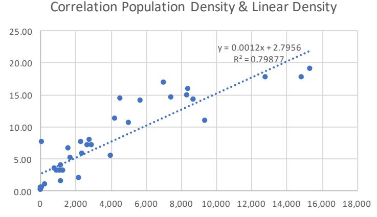
Figure 6. Pearson correlation of population density and linear density of the 34 Indonesian provincial capitals. Source: Author, 2020

Table 3 shows the differences between the groups of cities from the six regions based on mean administrative area size, mean linear density, mean population size, and mean population density. The mean administrative sizes of the cities in Sumatra and Java-Bali are fairly similar, between 270 and 280 km² , whereas the two cities in Nusa Tenggara have the smallest administrative size, at 120 km² . According to the table, the administrative areas of the cities from Sumatra, Java-Bali and Nusa Tenggara are smaller in size than those from Kalimantan, Sulawesi, and Maluku-Papua, where cities have developed more recently and on more easily available land. Consequently, whereas cities from Kalimantan, Sulawesi, and Maluku-Papua have a larger administrative area, they also have lower mean linear density, population, and population density than the cities in Sumatra, Java-Bali, and Nusa Tenggara.

Table 3. Regional variations of the 34 Indonesian cities' geometrical value, population, and density.

Regional Zone	Mean administrative area km2	Mean linear density	Mean population	Mean population density/km2
Sumatra	287.80	7.92	841,614.40	3,275.40
Java-Bali	279.60	14.57	2,727,416.86	9,369.43
Nusa Tenggara	120.79	8.19	430,800.00	4,862.50
Kalimantan	856.11	5.75	499,105.00	3,293.20
Sulawesi	1,025.69	5.98	492,510.67	2,709.83
Maluku-Papua	1,126.68	2.47	220,270.25	408.00

The ANOVA test for linear density and population density comparing the six regional groups (Sumatra, Java-Bali, Nusa Tenggara, Kalimantan, Sulawesi, and Maluku-Papua) is shown in Table 4. For these variables, the differences between the regions are statistically significant.

Table 4. ANOVA test on global integration and connectivity of the six regional groups.

ANOVA test Sum of Squares df Mean Square F Sig. Linear density Between groups 474.002 5 94.800 3.815 .009 Within groups 695.852 28 24.852 Total 1169.855 33 Built-up area density Between groups .252 5 .050 8.640 .000 Within groups .164 28 .006 Total .416 33

3.2. Indonesian City Shape Patterns

The study of the patterns of city shapesin this research used OSMnx to quantify order and disorder of street network angularity using entropy. Entropy helps identify if a city is formal in nature, with a value closer to 1.0 for a strongly gridded street network and a value closer to 0.1 if it is more natural/organic and has diverse and complex street angularity orientations (Boeing, 2019; Romdhoni & Rashid, 2019). According to the findings of this study, there are regional variations in street angularity orientation as represented by the distinctive polar histograms of the cities from these regions, which are described below.

Sumatra region: The ten case study cities form this region are: Banda Aceh, Medan, Padang, Pekanbaru, Jambi, Palembang, Bengkulu, Bandar Lampung, Pangkal Pinang, and Tanjung Pinang. With their polar graphs showing street orientations in each of the 36 bins, most cities from this region have natural growth patterns. In contrast, Medan and Banda Aceh are the only cities with polar graphs showing very rigid street orientations, with N-S and E-W being the predominant directions. The mean entropy grid value for this region is 0.54.

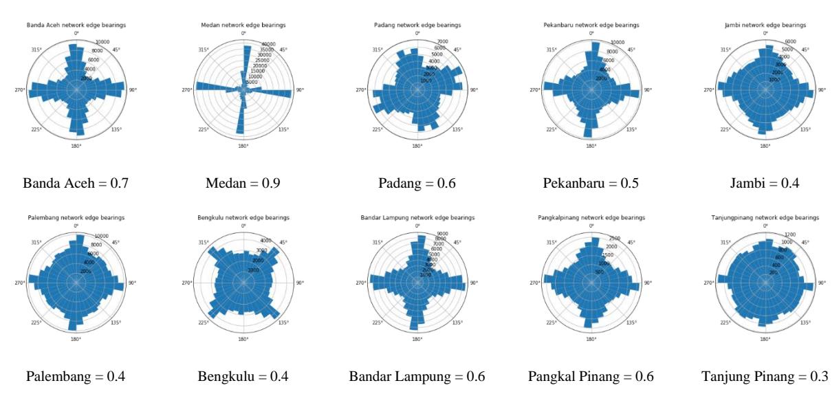
Figure 7. Sumatra region street network shape patterns and grid values.

Java-Bali region: The seven case study cities from this region are: Jakarta, Bandung, Semarang, Yogyakarta, Surabaya, Serang, and Denpasar. These cities are grid-like with different values for griddedness. The polar graphs of the cities from this region show consistent street orientations along two predominant directions. The mean entropy value for this region is 0.79

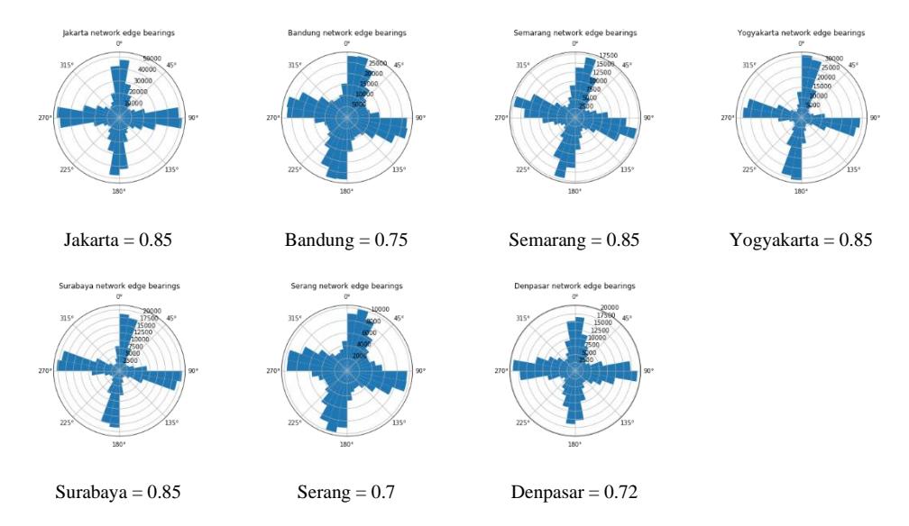
Figure 8. Java-Bali region street network shape patterns and grid values.

Nusa Tenggara region: The two capital cities from this region are Mataram and Kupang. The polar diagrams of these cities show a mixture of grid and organic city patterns. The grid entropy value is 0.6 for Kupang and 0.7 for Mataram. The mean entropy grid value for this region is 0.65.

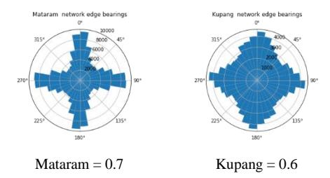
Figure 9. Nusa Tenggara region street network shape patterns and grid values.

Kalimantan region: The five case study cities from this region are: Pontianak, Palangkaraya, Banjarmasin, Samarinda, Tanjung Selor. Three of the case study cities are rather unique, showing a superimposed grid pattern (Pontianak, Palangkaraya, and Banjarmasin) not seen in the other Indonesian case study cities. Palangkaraya is a special case because it was originally designed to be the capital city of the nation under Indonesia's first president Sukarno. The city was planned with eight special axes. However, the capital city of Indonesia was never moved from Jakarta; Palangkaraya now functions as the provincial ca pital of Central Kalimantan. The entropy grid value for this group of cities from the Kalimantan region varies between 0.4 and 0.86.

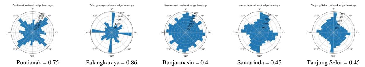
Figure 10. Kalimantan region street network shape patterns and grid values.

Sulawesi region: The study sample included six coastal cities from this region, i.e., Manado, Palu, Makassar, Kendari, Gorontalo, and Mamuju. The polar diagrams of these cities show some of them as strongly gridded cities, while the rest are organic cities. The entropy grid value for the Sulawesi region varies between 0.3 and 0.86.

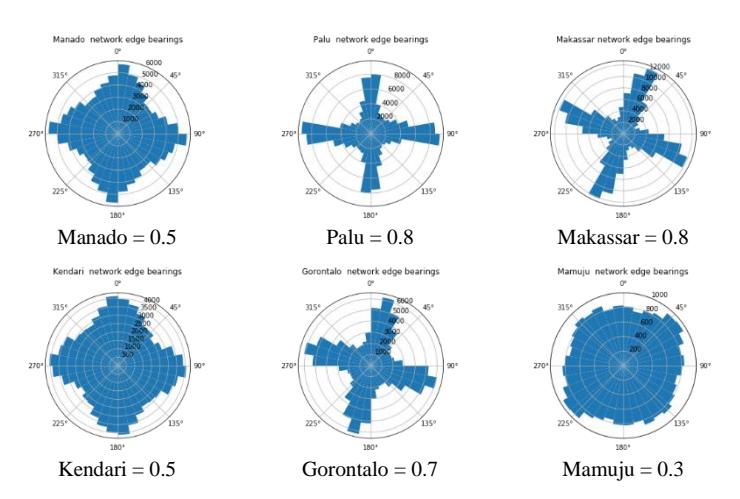
Figure 11. Sulawesi region street network shape patterns and grid values.

Maluku-Papua: The four case study cities in this region are Ambon, Sofifi, Jayapura, and Manokwari. The polar diagrams of these cities show natural patterns of growth with their streets having no predominant directions. The grid entropy value for Maluku-Papua region varies between 0.35 and 0.4. The mean entropy grid value for this region is 0.387, indicating a more natural street network pattern. The mean value of grid entropy is the lowest compared to the other regions in Indonesia. It is also important to mention that this region has been less developed compared to the other five regions of Indonesia included in this study.

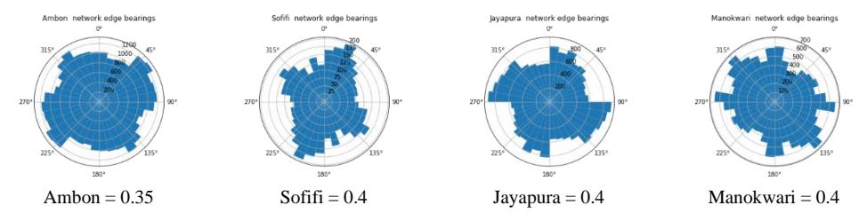
Figure 12. Maluku-Papua region street network shape pattern and grid value

The street network orientation method is unique for its ability to describe the angularity patterns of street networks. The finding of this study shows regional variations among the 34 case study cities. The mean grid entropy values of these regions are Sumatra = 0.540, Java-Bali = 0.795, Nusa Tenggara = 0.65, Kalimantan = 0.582, Sulawesi = 0.6, and Maluku-Papua = 0.388.

According to this study, the mean grid entropy values of the cities in the different regions are consistent with the polar histograms provided above. Both the polar histogram and the grid entropy values show that Java-Bali cities have a more consistent grid form compared to the cities from the other regions of Indonesia, while the cities in Maluku-Papua have a value consistent with naturally formed cities, with streets showing no predominant direction.

Table 5. Grid entropy one-way ANOVA mean test value of the six regional groups.

Grid entropy ANOVA of the six regional groups

	Sum of Squares	df	Mean Square	F	Sig.
Between Groups	.491	5	.098	3.969	.008
Within Groups	.693	28	.025
Total	1.184	33

There is a statistically significant difference between the six regional groups of the 34 case study cities as demonstrated by the one-way ANOVA test (p = .008).

3.3. Indonesian Cities Street Network Movement

The digitized axial maps of 900 square kilometers from the case study cities were analyzed using Axwoman 6.3. and ArcMap 10.4. Figure 13 provides colored axial maps of the Indonesian provincial capitals that show the line hierarchy using the global integration value. The colored maps also allowed us to identify the syntactic cores of these cities defined by the most integrated set of streets, which were also defined as the foreground structure of these cities. The types of syntactic cores found in this study were: (1) tree type structure (Banda Aceh, Padang, Jambi, Pangkal Pinang, Tanjung Pinang, Semarang, Serang, Kupang, Banjarmasin, Samarinda, Tanjung Selor, Manado, Palu, Makassar, Mamuju, Ambon, Sofifi, Jayapura, Manokwari); (2) grid structure (Gorontalo); (3) deformed wheel structure (Palembang, Bandar Lampung, Jakarta, Bandung, Kendari); and (4) super grid structure (Medan, Pekanbaru, Bengkulu, Yogyakarta, Surabaya, Denpasar, Mataram, Pontianak, Palangkaraya). These different types of syntactic cores or foreground structures indicate that the economy of space may work differently in these cities (Rashid, 2021). For example, in cities with supergrids, global movement gets priority over local accessibility, whereas in cities with grid structures, global movement and local accessibility find a balance.

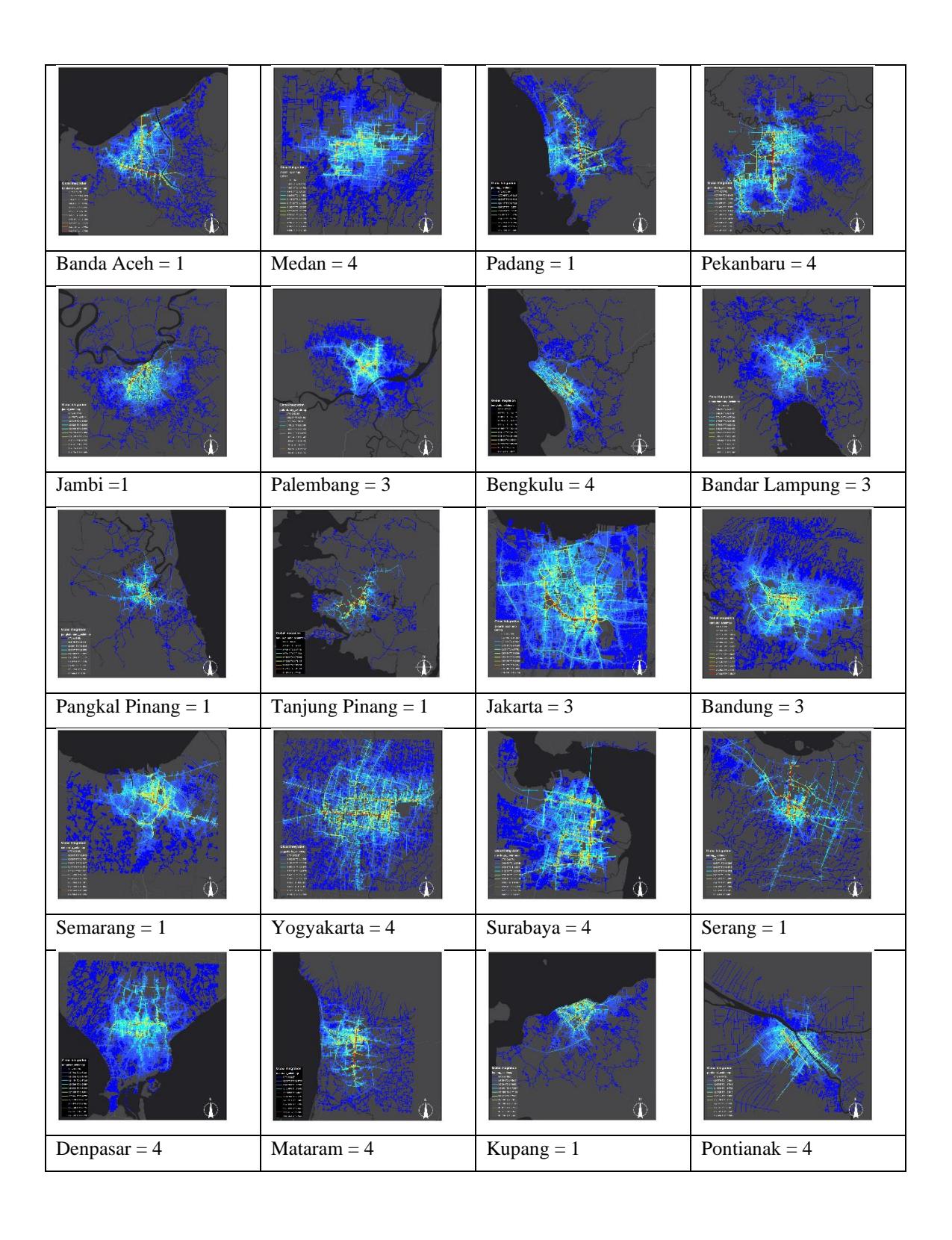
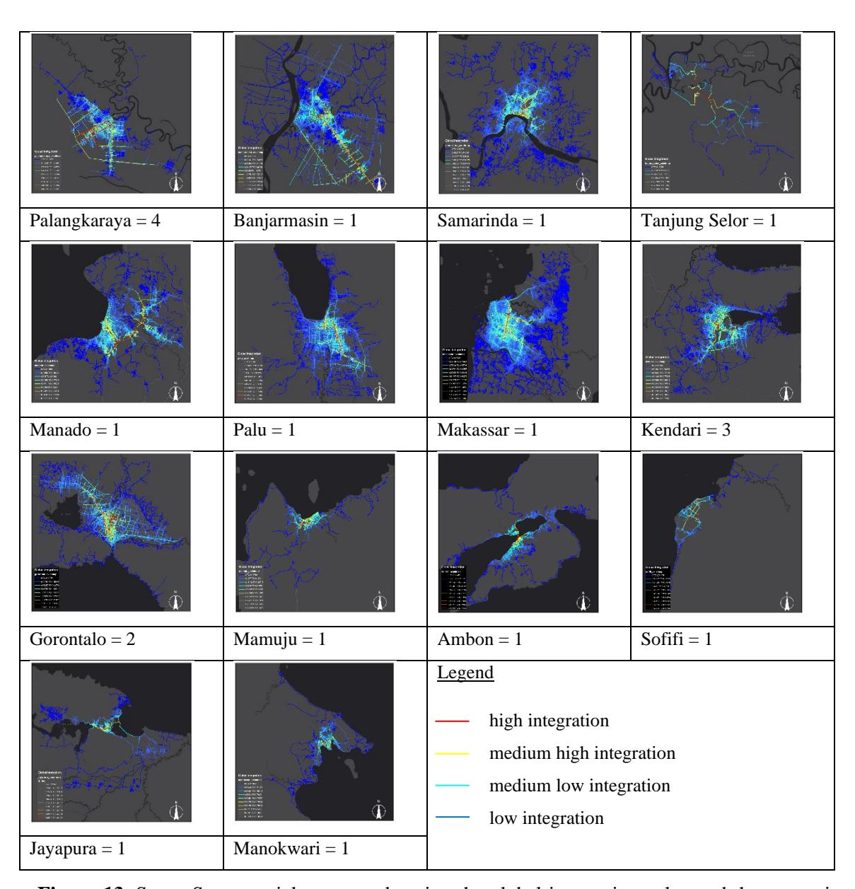
Figure 13. Space Syntax axial maps made using the global integration value and the syntactic core of 34 Indonesian provincial capitals. Source: Author, 2020.

The global integration values from the axial maps of the case study cities show variations, indicating that the cities in the eastern part of Indonesia have less integrated street networks than those in the central and western parts of Indonesia. The findings also show that Yogyakarta in the Java-Bali region and Palangkaraya in the Kalimantan region have the highest mean integration values. The findings, shown in Figure 14, show the value of minimum, maximum, and mean integration values for the 34 Indonesian provincial capitals.

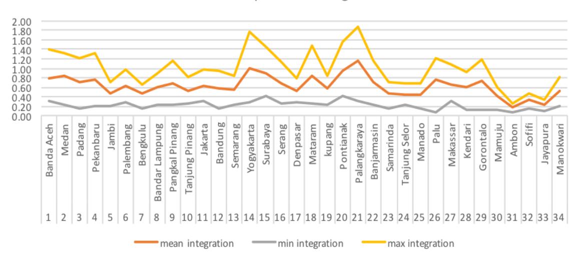
Figure 14. Histogram of axial map global integration for the 34 provincial capitals. Source: Author, 2020

Table 6 shows the regional differences in the axial map analysis of the 34 case study cities grouped within their respective regions. The seven cities from the region of Java-Bali have the highest mean number of axial segments of 40,826 within 900 km² . The mean integration in Java-Bali is 0.696 with a minimum integration of 0.271 and a maximum integration of 1.129. The high value of mean integration in this region is an indication of high movement potential in the urban areas of these cities. In contrast, the four cities from the region of Maluku-Papua have the lowest number of axial segments at only 2241 axial lines within 900 km² . The mean integration in Maluku-Papua is only 0.315, with a range of integration value from 0.125 to 0.470. The low value of mean integration in this region is an indication of low movement potential in the urban areas of these cities.

Table 6. Regional variations between the 34 Indonesian cities' integration value, min, mean, max,
and connect.

Regional zone	Mean number axial map segment	Mean	Min	Max
		integration	integration	integration
Sumatra	19,833	0.646	0.222	1.045
Java-Bali	40,826	0.696	0.271	1.129
Nusa Tenggara	10,324	0.700	0.235	1.160
Kalimantan	7,164	0.740	0.266	1.200
Sulawesi	10,044	0.597	0.153	0.948
Maluku-Papua	2,241	0.315	0.125	0.470

ANOVA was used to find out if the differences in mean integration are significant among the cities from the six different regions. Along with the ANOVA test, Levene's test of homogeneity of means was also conducted. The p value of Levene's test for the three variables (mean, max, and min integration) were higher than the significance level (p < 0.05), showing that the variances were equal and hence satisfy the condition for the ANOVA test.

Table 7. Test of homogeneity of variances on global integration and connectivity of the six regional groups.

	Levene's	df1	df2	Sig.
	statistic
Mean integration	1.825	5	28	.140
Max integration	1.546	5	28	.208
Min integration	.951	5	28	.464

Table 8 shows the result of the ANOVA test for mean integration, maximum integration, and minimum integration of the space syntax method for the six regional groups (Sumatra, Java-Bali, Nusa Tenggara, Kalimantan, Sulawesi, and Maluku-Papua). These variables showed statistically significant differences between the regions.

Table 8. ANOVA test on global integration and connectivity of the six regional groups.

ANOVA

		Sum of Squares	df	Mean Square	F	Sig.
Mean integration	Between groups	.506	5	.101	2.998	.027
	Within groups	.945	28	.034
	Total	1.451	33
Max integration	Between groups	1.525	5	.305	2.588	.048
	Within groups	3.300	28	.118
	Total	4.825	33
Min integration	Between groups	.092	5	.018	3.345	.017
	Within groups	.154	28	.005
	Total	.245	33

4. Discussion

The purpose of this study was to explore the regional variations of the morphology of Indonesian cities using provincial capital cities as case studies. We used recent datasets and techniques provided in the literature to obtain an accurate descriptive model. The spatial datasets and techniques included in this study were: (1) OpenStreetMap (OSM) street centerlines with geometric properties, (2) Landsat and Google map GeoTiff earth surface images to understand the built-up area density of the case study cities, and (3) digitized axial segment for axial space syntax analysis to understand the Indonesian provincial capital cities' topological structures.

OSM's street centerline dataset was essential for this study to understand the geometric properties and to measure the entropy in street grids, giving a better understanding of the urban street angularity. Landsat and Google map GeoTiff earth surface images for each city were also used to understand the general land cover index, complementing other urban density information. The axial segment map dataset was digitized using ArcMap 10.4. software and provided robust space syntax indicators, such as global integration, and foreground and background networks, revealing each case study cities' syntactic core patterns.

Further analysis, as shown in Table 9, revealed a strong correlation between the spatial griddedness of OSMnx and the global integration of space syntax for the 34 case study cities. The Pearson correlation between the mean global integration and the grid entropy value was 0.705 or the coefficient of determination R² = 0.4972 with the two-tailed significance p-value = .001. Put

simply, different geometric properties of these cities appear to be strongly interrelated. The Pearson correlation between grid value and mean integration was also strong, with a value of 0.635 with the two-tailed significance p-value = .001 and 0.397 with the two-tailed significance p-value = .005.


	Correlations
		1	2	3	4
1. Grid value	Pearson correlation
	Sig. (two-tailed)
2. Mean integration	Pearson correlation	.705**
	Sig. (two-tailed)	0
3. Linear density	Pearson correlation	.635**	.397*
	Sig. (two-tailed)	0	0.02
4. Built-up area density	Pearson correlation	.369*	0.118	.461**
	Sig. (two-tailed)	0.032	0.505	0.006
5. Population density/km2	Pearson correlation	.582**	.370*	.894**	.473**
	Sig. (two-tailed)	0	0.031	0	0.005

Table 9. Multiple correlational analysis. Source: Author, 2021

Tukey's post hoc test was also conducted (Table 10) to find out if there were significant differences among cities between any two groups. The results showed significant differences between the Java-Bali and Maluku-Papua regions (p = .004), and between the Sumatra and Java-Bali regions (p = .029). The cities from the Nusa Tenggara, Kalimantan, and Sulawesi regions showed no significant difference with the other regions. Significant differences also appeared in the mean integration from the topologic space syntax findings. The result showed significant differences between the Sumatra and Malulu-Papua regions (p = .051), between the Java-Bali and Maluku-Papua regions (p = .028), and between the Kalimantan and Maluku-Papua regions (p = .020).

The Tukey's post hoc test showed significant differences between cities in their respective regions in linear density, built-up area density, and population density variables. The linear density in Indonesian cities regionally showed significant differences within the Java-Bali and Kalimantan regions (p = .054), the Sulawesi region (p = 0.46), and the Maluku-Papua region (p = .007). The built-up area density using remote sensing confirmed that Java-Bali is significantly different in this respect from the other regions, i.e., Sumatra (p = .001), Nusa Tenggara (p = .003), Kalimantan (p= .001), Sulawesi (p = .001), and Maluku-Papua (p = .001). Population density is also significantly different between the cities in the Java-Bali region from those in the Sumatra region (p = .015), the Sulawesi region (p = .019), and the Maluku-Papua region (p = .004).

^**Correlation is significant at the 0.01 level (two-tailed).

^*Correlation is significant at the 0.05 level (two-tailed).

					Significant p-value
Dependent	(I) Regional	(J) Regional	Grid	Mean	Linear	Built	Popula
Variable	Group	Group	value	integra	density	up area	tion
		Group		tion		density	density
		Java-Bali	.029	.993	.105	.001	.015
	Sumatra	Nusa Tenggara	.943	.999	1.000	.710	.991
		Kalimantan	.996	.934	.966	.927	1.000
		Sulawesi	.975	.995	.973	.845	1.000
		Maluku-Papua	.581	.051	.455	.772	.724
		Nusa Tenggara	.854	1.000	.608	.003	.588
		Kalimantan	.220	.998	.054	.001	.056
Indonesia's six	Java-Bali	Sulawesi	.254	.924	.046	.000	.019
regions		Maluku-Papua	.004	.028	.007	.001	.004
		Kalimantan	.995	1.000	.991	.981	.994
	Nusa	Sulawesi	.999	.982	.994	.989	.971
	Tenggara	Maluku-Papua	.408	.184	.769	.999	.673
		Sulawesi	1.000	.789	1.000	1.000	1.000
	Kalimantan	Maluku-Papua	.456	.020	.920	.999	.811
	Sulawesi	Maluku-Papua	.320	.199	.882	1.000	.903

Table 10. Multiple comparisons of Tukey's post hoc test in the research findings.

Performed using the GIS software, the techniques used in this study provided a robust workflow to understand the urban geometries and spatial patterns of Indonesian cities in different regions. The study's findings showed that there are regional variations among Indonesian provincial capitals. The findings on the spatial patterns of street networks suggest that the Java-Bali, Sumatra, and Maluku-Papua regions have statistically significant differences in 1) street orientation defined by the grid value, 2) collective movement defined by integration, 3) linear density, 4) built-up area density, and 5) population density size.

The findings showed statistically significant differences between the Java-Bali and Maluku-Papua regions for all variables. The reasons for the differences are clear. The cities in Java-Bali generally have a formal spatial pattern due to more colonial influences and more modern development, whereas the cities in Maluku-Papua have natural spatial patterns due to less colonial influence and less modern development. The cities in Kalimantan showed a significant statistical difference from the cities in Java-Bali in linear density and built-up area density. Additionally, the geometric form of the street patterns in the Kalimantan provincial capitals showed a consistent superimposed grid layout that differs from the other regions (Figure 10). The findings indicate that the proposed capital in Kalimantan may need to be different from Jakarta if it wants to remain sensitive to the regional patterns found in Kalimantan.

5. Conclusion

The four major findings of this study are: 1) VGI data sources can be utilized using Python extraction methods to understand the geometric properties of street networks of Indonesian cities. 2) Geometric properties, street orientation patterns and the topological structure of street networks are often correlated in Indonesian cities. For example, the cities' griddedness is strongly correlated with topological measures such as global integration. To put it differently, cities with a formal gridded pattern usually have higher integration values compared to those with an organic and natural pattern. 3) The findings on the spatial patterns indicate that the cities in the Java-Bali region generally have a more formal street network, showing highly gridded patterns, while the

^*The mean difference is significant at the 0.05 level.

other regions have a mixture of gridded and natural patterns. The cities in the Maluku-Papua region consistently show a natural form based on street orientation. 4) The classical city model of Indonesian cities and colonial port cities shows a concentric pattern with a central point that generally served as port or government center. Current Indonesian cities, however, show variations in spatial structures. There is no longer a single center in these cities, rather, there are syntactic cores of different shapes, i.e., tree, grid, deformed wheel, and supergrid, which serve the cities differently. This study suggests that regional variations among Indonesian cities may have been due to differences in modern development patterns. Further study is needed to confirm the results reported here. This study of 34 Indonesian cities hopes to provide a benchmark for future geometric studies on Indonesian cities. It may benefit urban studies in other developing countries where there is a lack of resources to conduct large-scale comparative studies.

Research Intelligence

Data from OpenAlex ↗

Metrics

1

Citations

0.11

FWCIfield-weighted

44th

Percentilevs same year + field

Article

Work type

DIAMOND

Open Access

Topics

Urban Design and Spatial Analysis Primary

0.97

Building and Construction › Engineering › Physical Sciences

Remote Sensing and Land Use

0.93

Related Research

Citation Trend

1

2024

Citation Timeline

Year	Citations
2024	1

Semantic Profile AI-classified research signals

Core Domains

Geography 0.78

level 0

Indonesian 0.62

level 2

Regional science 0.52

level 1

Secondary Topics

Economic geography 0.46 Population 0.42 Cartography 0.39

Institution Network

Sriwijaya University ID
Muhammad Fajri Romdhoni
University of Kansas US
Mahbub Rashid

References

Barron, C., Neis, P., & Zipf, A. (2014). A comprehensive framework for intrinsic OpenStreetMap quality analysis. Transactions in GIS, 18(6), 877–895.
Boeing, G. (2017). OSMnx: New methods for acquiring, constructing, analyzing, and visualizing complex street networks. Computers, Environment and Urban Systems, 65, 126–139.
Boeing, G. (2019). Urban spatial order: Street network orientation, configuration, and entropy. Applied Network Science, 4(1), 67. DOI: 10.1007/s41109-019-0189-1
Bowden, M. J. (1972). The Internal Structure of the Colonial Replica City: San Francisco and Others. Unpublished Paper Presented to the Annual Conference of the Association of American Geographers, Kansas City.
Chen, X. (2018). A Comparative Study of the Supergrid and Superblock Structures in Chinese and Japanese Cities. International Journal of the Constructed Environment, 9(3). DOI: 10.18848/2154-8587/cgp/v09i03/45-63
Chen, X. F. (2018). Spatial Structure in Chinese and Japanese Cities: A Comparative Study of the Supergrid and Superblock Structure. 24th ISUF International Conference. Book of Papers, 125–137. DOI: 10.18848/2154-8587/cgp/v09i03/45-63
Field, A. (2007). Analysis of variance (ANOVA). Encyclopedia of Measurement and Statistics, 33–36.
Ford, L. R. (1993). A model of Indonesian city structure. Geographical Review, 374–396. DOI: 10.2307/215821
Girres, J.-F., & Touya, G. (2010). Quality assessment of the French OpenStreetMap dataset. Transactions in GIS, 14(4), 435–459.
Haklay, M. (2010). How good is volunteered geographical information? A comparative study of OpenStreetMap and Ordnance Survey datasets. Environment and Planning B: Planning and Design, 37(4), 682–703. DOI: 10.1068/b35097
Hillier, B. (2005). The art of place and the science of space. World Architecture, 185, 96–102.
Hillier, B. (2007). Space is the machine: A configurational theory of architecture. Space Syntax.
Hillier, B. (2008). Space and spatiality: What the built environment needs from social theory. Building Research & Information, 36(3), 216–230. DOI: 10.1080/09613210801928073
Hillier, B. (2012a). Studying cities to learn about minds: Some possible implications of space syntax for spatial cognition. Environment and Planning B: Planning and Design, 39(1), 12–32. DOI: 10.1068/b34047t
Hillier, B. (2012b). The city as a socio-technical system: A spatial reformulation in the light of the levels problem and the parallel problem. In Digital Urban Modeling and Simulation (pp. 24–48). Springer. DOI: 10.1007/978-3-642-29758-8_3
Hillier, B. (2016). What are cities for? And how does it relate to their spatial form? The Journal of Space Syntax, 6(2), 199–212.
Hillier, B. H., & Hanson, J. (1984). J. 1984 The Social Logic of Space. Cambridge University.
Hillier, B., & Hanson, J. (1989). The social logic of space. Cambridge university press.
Hillier, B., & Iida, S. (2005). Network and psychological effects in urban movement. International Conference on Spatial Information Theory, 475–490. DOI: 10.1007/11556114_30
Hillier, B., Leaman, A., Stansall, P., & Bedford, M. (1976). Space syntax. Environment and Planning B: Planning and Design, 3(2), 147–185.
Hornsby, S. J. (1997). Discovering the mercantile city in South Asia: The example of early nineteenth-century Calcutta. Journal of Historical Geography, 23(2), 135–150. DOI: 10.1006/jhge.1996.0046
Jiang, B. (2015). Axwoman 6.3: An ArcGIS extension for urban morphological analysis. University of Gävle, Sweden.
Jiang, B. (2019). Axwoman in a Nutshell.
Jones, G. W., & Mulyana, W. (2015). Urbanization in Indonesia: UNFPA Indonesia Monograph Series No. 4. Jakarta: UNFPA.
Joseph, M., Wang, L., & Wang, F. (2012). Using Landsat imagery and census data for urban population density modeling in Port-au-Prince, Haiti. GIScience & Remote Sensing, 49(2), 228–250. DOI: 10.2747/1548-1603.49.2.228
Kosambi, M., & Brush, J. E. (1988). Three colonial port cities in India. Geographical Review, 32–47. DOI: 10.2307/214304
Kruger, M. J. T. (1989). On node and axial grid maps: Distance measures and related topics.
Law, S., Chiaradia, A., & Schwander, C. (2012). Towards a multimodal space syntax analysis: A case study of the London street and underground network. Published in Proceedings of the 8th International Space Syntax Symposium, Santiago de Chile, Chile, 36.
Li, G., & Weng, Q. (2005). Using Landsat ETM+ imagery to measure population density in Indianapolis, Indiana, USA. Photogrammetric Engineering & Remote Sensing, 71(8), 947–958. DOI: 10.14358/pers.71.8.947
Minaei, M. (2020). Evolution, density and completeness of OpenStreetMap road networks in developing countries: The case of Iran. Applied Geography, 119, 102246. DOI: 10.1016/j.apgeog.2020.102246
Nations, U. (2018). The World’s Cities in 2018. https://www.un-ilibrary.org/content/publication/c93f4dc6-en
Oliveira, V., Monteiro, C., & Partanen, J. (2015). A comparative study of urban form. Urban Morphology, 19(1), 73–92.
Park, J.-M., Yang, S.-J., & Lee, H.-H. (2014). Transition of Jinhae’s Urban Spatial Configuration Analysed by Space Syntax. Journal of the Architectural Institute of Korea Planning & Design, 30(11), 89–96.
Peponis, J., Hadjinikolaou, E., Livieratos, C., & Fatouros, D. A. (1989). The spatial core of urban culture. Ekistics, 43–55.
Rashid, M. (2017). The Geometry of Urban Layouts. DOI: 10.1007/978-3-319-30750-3
Rashid, M. (2019). Space Syntax: A Network-Based Configurational Approach to Studying Urban Morphology. In The Mathematics of Urban Morphology (pp. 199–251). Springer. DOI: 10.1007/978-3-030-12381-9_10
Rashid, M. (2021). Physical Space and Spatiality in Muslim Societies: Notes on the Social Production of Cities. University of Michigan Press.
Rashid, M., & Shateh, H. (2012). The dialectics of functional and historical morphology in the evolution of a city: The case of the Stone Town of Zanzibar. The Journal of Architecture, 17(6), 889–924. DOI: 10.1080/13602365.2012.746009
Roberts, M., Sander, F. G., & Tiwari, S. (2019). Time to ACT: Realizing Indonesia’s Urban Potential. World Bank Publications. DOI: 10.1596/978-1-4648-1389-4
Romdhoni, M. F. (2020). Understanding The Urban Population Density and Growth Concentration in Palembang Indonesia. Journal of Architecture&ENVIRONMENT, 19(2), 187–204. DOI: 10.12962/j2355262x.v19i2.a7510
Romdhoni, M. F., & Rashid, M. (2019). Street Angularity and Patterns in Palembang and Yogyakarta, Indonesia. Proceedings of Indonesia Focus, 1(1).
Shannon, C. E. (1948). A mathematical theory of communication. Bell System Technical Journal, 27(3), 379–423. DOI: 10.1002/j.1538-7305.1948.tb01338.x
Siksna, A. (1998). City centre blocks and their evolution: A comparative study of eight American and Australian CBDs. Journal of Urban Design, 3(3), 253–283. DOI: 10.1080/13574809808724429
Sun, X. (2013). Comparative analysis of urban morphology: Evaluating space syntax and traditional morphological methods.
Sunaryo, R. G., Soewarno, N., & Setiawan, B. (2012). Morphological study of colonial and traditional urban space in Java: A comparative study of ten cities [PhD Thesis]. Petra Christian University.
Turner, A. (2007). From axial to road-centre lines: A new representation for space syntax and a new model of route choice for transport network analysis. Environment and Planning B: Planning and Design, 34(3), 539–555. DOI: 10.1068/b32067
Turner, A., Penn, A., & Hillier, B. (2005). An algorithmic definition of the axial map. Environment and Planning B: Planning and Design, 32(3), 425–444. DOI: 10.1068/b31097
Tutuko, P., Bonifacius, N., Yuniawan, D., Junianto, M. R., & Telnoni, R. J. A. (2018). Colonial city pattern in Indonesia using depth calculation: Introduction to study ratio on master plans using DepthMapX. ICIAP International Conference on Indonesian Architecture and Planning: Design and Planning in the Disruptive Era, 634–641.
Widodo, J. (2004). The Boat and the City: Chinese Diaspora and the Architecture of Southeast Asian Coastal Cities. Marshall Cavendish Academic.
Zielstra, D., Hochmair, H. H., & Neis, P. (2013). Assessing the Effect of Data Imports on the Completeness of OpenStreetMap – A United States Case Study. Transactions in GIS, 17(3), 315–334.

Download PDF

[ref-1] Barron, C., Neis, P., & Zipf, A. (2014). A comprehensive framework for intrinsic OpenStreetMap quality analysis. Transactions in GIS, 18(6), 877–895.

[ref-2] Boeing, G. (2017). OSMnx: New methods for acquiring, constructing, analyzing, and visualizing complex street networks. Computers, Environment and Urban Systems, 65, 126–139.

[ref-3] Boeing, G. (2019). Urban spatial order: Street network orientation, configuration, and entropy. Applied Network Science, 4(1), 67. DOI: 10.1007/s41109-019-0189-1

[ref-4] Bowden, M. J. (1972). The Internal Structure of the Colonial Replica City: San Francisco and Others. Unpublished Paper Presented to the Annual Conference of the Association of American Geographers, Kansas City.

[ref-5] Chen, X. (2018). A Comparative Study of the Supergrid and Superblock Structures in Chinese and Japanese Cities. International Journal of the Constructed Environment, 9(3). DOI: 10.18848/2154-8587/cgp/v09i03/45-63

[ref-6] Chen, X. F. (2018). Spatial Structure in Chinese and Japanese Cities: A Comparative Study of the Supergrid and Superblock Structure. 24th ISUF International Conference. Book of Papers, 125–137. DOI: 10.18848/2154-8587/cgp/v09i03/45-63

[ref-7] Field, A. (2007). Analysis of variance (ANOVA). Encyclopedia of Measurement and Statistics, 33–36.

[ref-8] Ford, L. R. (1993). A model of Indonesian city structure. Geographical Review, 374–396. DOI: 10.2307/215821

[ref-9] Girres, J.-F., & Touya, G. (2010). Quality assessment of the French OpenStreetMap dataset. Transactions in GIS, 14(4), 435–459.

[ref-10] Haklay, M. (2010). How good is volunteered geographical information? A comparative study of OpenStreetMap and Ordnance Survey datasets. Environment and Planning B: Planning and Design, 37(4), 682–703. DOI: 10.1068/b35097

[ref-11] Hillier, B. (2005). The art of place and the science of space. World Architecture, 185, 96–102.

[ref-12] Hillier, B. (2007). Space is the machine: A configurational theory of architecture. Space Syntax.

[ref-13] Hillier, B. (2008). Space and spatiality: What the built environment needs from social theory. Building Research & Information, 36(3), 216–230. DOI: 10.1080/09613210801928073

[ref-14] Hillier, B. (2012a). Studying cities to learn about minds: Some possible implications of space syntax for spatial cognition. Environment and Planning B: Planning and Design, 39(1), 12–32. DOI: 10.1068/b34047t

[ref-15] Hillier, B. (2012b). The city as a socio-technical system: A spatial reformulation in the light of the levels problem and the parallel problem. In Digital Urban Modeling and Simulation (pp. 24–48). Springer. DOI: 10.1007/978-3-642-29758-8_3

[ref-16] Hillier, B. (2016). What are cities for? And how does it relate to their spatial form? The Journal of Space Syntax, 6(2), 199–212.

[ref-17] Hillier, B. H., & Hanson, J. (1984). J. 1984 The Social Logic of Space. Cambridge University.

[ref-18] Hillier, B., & Hanson, J. (1989). The social logic of space. Cambridge university press.

[ref-19] Hillier, B., & Iida, S. (2005). Network and psychological effects in urban movement. International Conference on Spatial Information Theory, 475–490. DOI: 10.1007/11556114_30

[ref-20] Hillier, B., Leaman, A., Stansall, P., & Bedford, M. (1976). Space syntax. Environment and Planning B: Planning and Design, 3(2), 147–185.

[ref-21] Hornsby, S. J. (1997). Discovering the mercantile city in South Asia: The example of early nineteenth-century Calcutta. Journal of Historical Geography, 23(2), 135–150. DOI: 10.1006/jhge.1996.0046

[ref-22] Jiang, B. (2015). Axwoman 6.3: An ArcGIS extension for urban morphological analysis. University of Gävle, Sweden.

[ref-23] Jiang, B. (2019). Axwoman in a Nutshell.

[ref-24] Jones, G. W., & Mulyana, W. (2015). Urbanization in Indonesia: UNFPA Indonesia Monograph Series No. 4. Jakarta: UNFPA.

[ref-25] Joseph, M., Wang, L., & Wang, F. (2012). Using Landsat imagery and census data for urban population density modeling in Port-au-Prince, Haiti. GIScience & Remote Sensing, 49(2), 228–250. DOI: 10.2747/1548-1603.49.2.228

[ref-26] Kosambi, M., & Brush, J. E. (1988). Three colonial port cities in India. Geographical Review, 32–47. DOI: 10.2307/214304

[ref-27] Kruger, M. J. T. (1989). On node and axial grid maps: Distance measures and related topics.

[ref-28] Law, S., Chiaradia, A., & Schwander, C. (2012). Towards a multimodal space syntax analysis: A case study of the London street and underground network. Published in Proceedings of the 8th International Space Syntax Symposium, Santiago de Chile, Chile, 36.

[ref-29] Li, G., & Weng, Q. (2005). Using Landsat ETM+ imagery to measure population density in Indianapolis, Indiana, USA. Photogrammetric Engineering & Remote Sensing, 71(8), 947–958. DOI: 10.14358/pers.71.8.947

[ref-30] Minaei, M. (2020). Evolution, density and completeness of OpenStreetMap road networks in developing countries: The case of Iran. Applied Geography, 119, 102246. DOI: 10.1016/j.apgeog.2020.102246

[ref-31] Nations, U. (2018). The World’s Cities in 2018. https://www.un-ilibrary.org/content/publication/c93f4dc6-en

[ref-32] Oliveira, V., Monteiro, C., & Partanen, J. (2015). A comparative study of urban form. Urban Morphology, 19(1), 73–92.

[ref-33] Park, J.-M., Yang, S.-J., & Lee, H.-H. (2014). Transition of Jinhae’s Urban Spatial Configuration Analysed by Space Syntax. Journal of the Architectural Institute of Korea Planning & Design, 30(11), 89–96.

[ref-34] Peponis, J., Hadjinikolaou, E., Livieratos, C., & Fatouros, D. A. (1989). The spatial core of urban culture. Ekistics, 43–55.

[ref-35] Rashid, M. (2017). The Geometry of Urban Layouts. DOI: 10.1007/978-3-319-30750-3

[ref-36] Rashid, M. (2019). Space Syntax: A Network-Based Configurational Approach to Studying Urban Morphology. In The Mathematics of Urban Morphology (pp. 199–251). Springer. DOI: 10.1007/978-3-030-12381-9_10

[ref-37] Rashid, M. (2021). Physical Space and Spatiality in Muslim Societies: Notes on the Social Production of Cities. University of Michigan Press.

[ref-38] Rashid, M., & Shateh, H. (2012). The dialectics of functional and historical morphology in the evolution of a city: The case of the Stone Town of Zanzibar. The Journal of Architecture, 17(6), 889–924. DOI: 10.1080/13602365.2012.746009

[ref-39] Roberts, M., Sander, F. G., & Tiwari, S. (2019). Time to ACT: Realizing Indonesia’s Urban Potential. World Bank Publications. DOI: 10.1596/978-1-4648-1389-4

[ref-40] Romdhoni, M. F. (2020). Understanding The Urban Population Density and Growth Concentration in Palembang Indonesia. Journal of Architecture&ENVIRONMENT, 19(2), 187–204. DOI: 10.12962/j2355262x.v19i2.a7510

[ref-41] Romdhoni, M. F., & Rashid, M. (2019). Street Angularity and Patterns in Palembang and Yogyakarta, Indonesia. Proceedings of Indonesia Focus, 1(1).

[ref-42] Shannon, C. E. (1948). A mathematical theory of communication. Bell System Technical Journal, 27(3), 379–423. DOI: 10.1002/j.1538-7305.1948.tb01338.x

[ref-43] Siksna, A. (1998). City centre blocks and their evolution: A comparative study of eight American and Australian CBDs. Journal of Urban Design, 3(3), 253–283. DOI: 10.1080/13574809808724429

[ref-44] Sun, X. (2013). Comparative analysis of urban morphology: Evaluating space syntax and traditional morphological methods.

[ref-45] Sunaryo, R. G., Soewarno, N., & Setiawan, B. (2012). Morphological study of colonial and traditional urban space in Java: A comparative study of ten cities [PhD Thesis]. Petra Christian University.

[ref-46] Turner, A. (2007). From axial to road-centre lines: A new representation for space syntax and a new model of route choice for transport network analysis. Environment and Planning B: Planning and Design, 34(3), 539–555. DOI: 10.1068/b32067

[ref-47] Turner, A., Penn, A., & Hillier, B. (2005). An algorithmic definition of the axial map. Environment and Planning B: Planning and Design, 32(3), 425–444. DOI: 10.1068/b31097

[ref-48] Tutuko, P., Bonifacius, N., Yuniawan, D., Junianto, M. R., & Telnoni, R. J. A. (2018). Colonial city pattern in Indonesia using depth calculation: Introduction to study ratio on master plans using DepthMapX. ICIAP International Conference on Indonesian Architecture and Planning: Design and Planning in the Disruptive Era, 634–641.

[ref-49] Widodo, J. (2004). The Boat and the City: Chinese Diaspora and the Architecture of Southeast Asian Coastal Cities. Marshall Cavendish Academic.

[ref-50] Zielstra, D., Hochmair, H. H., & Neis, P. (2013). Assessing the Effect of Data Imports on the Completeness of OpenStreetMap – A United States Case Study. Transactions in GIS, 17(3), 315–334.