
Introduction
In recent years, interconnected databases have enabled the use of big data. With the improvement of computational power and machine learning (ML), this technology has paved the way for applying ad hoc testing to all aspects of human life. Transportation is no exception to this trend. The industry has experienced a massive shift to the use of big data and data lakes in many applications, such as intelligent transportation systems (ITS) (Kaffash, Nguyen & Zhu, 2021), smart cities, and the Internet of Things (IoT) (Rathore, Ahmad, Paul & Rho, 2016; Rathore et al., 2018), vehicular communication (An & Wu, 2020), railway transportation systems (Ghofrani, He, Goverde & Liu, 2018), and transportation and logistics (Ayed, Halima & Alimi, 2015). Traditionally, census data, household travel, and activity surveys were the major data sources in travel demand modeling. However, travel and activity surveys are very time-consuming and expensive and only cover a small sample of the population, which may also be biased toward specific socioeconomic groups. Nowadays, public transportation stations, vehicles, and mobile phones increasingly and passively collect mobility data. Fortunately, pattern recognition (Bishop, 2006) enables us to distinguish travel behavior patterns from these passive travel data. The only issue here is somehow relating these massive travel data to socioeconomic characteristics without violating privacy. This study aimed to solve this problem by inferring and synthesizing probable socioeconomic characteristics from travel patterns.
Socioeconomic characteristics are among the factorsthat are of great importance in transportation modeling. These characteristics can include age, income, education, gender, and marital status and are usually gathered through conventional travel surveys using population synthesis or census data. Regarding travel demand modeling (TDM), household characteristics such as income and socioeconomic status can have a major influence on travel patterns and as a result can be useful in selecting efficient traffic management policies for transport planners (Gärling & Schuitema, 2007). Population groups are targeted to implement effective types of policies based on their socioeconomic characteristics. For example, low-income groups are more likely to be motivated to reduce private car use and turn to public transportation if road pricing is applied (Jakobsson, Fujii & Gärling, 2000). From a transport policy perspective, demographic information is important in outlining optimum urban transport strategies such as transport service levels and fares, considering the limited available resources (Shepherd et al., 2006).
There is ample evidence that people with different socioeconomic characteristics have different travel behaviors (Carlsson-Kanyama & Linden, 1999; Li, Lo & Guo, 2018). Travel behavior patterns are differentiated by gender, age, and race (Crane & Takahashi, 2009). For example, some studies have shown that men tend to have more business and work activities, while women have more leisure activities such as visiting relatives or meeting friends (Collins & Tisdell, 2002). Women tend to travel shorter, during off-peak hours, or use flexible modes (Ng & Acker, 2018). Income is also a factor that influences travel behavior; income level can alter travel patterns such as travel distance (Jain & Tiwari, 2019). Due to the similarities in travel patterns and mobility in different demographic groups, we hypothesized that age, income, and gender can be inferred and estimated using travel pattern data.
Over the past few years, several attempts have been made to investigate the association between travel behavior patterns and socioeconomic characteristics. For instance, (Zhu, Gonder & Lin, 2017) predicted individuals' sociodemographic characteristics based on continuously collected eighteen-month GPS data of 275 households, including employment status, age, gender, and income. They extracted home-based and non-home-based tours from raw GPS data, trained SVM and logistic regression, and concluded that SVM performed better in their case. Variables related to the spatiotemporal variability among tours were among the most important distinguishing factors they used for classification. Employment status was best estimated among studied sociodemographic roles. Although they gained high accuracy in their modeling, the proposed model needs to be applied to a larger data set to be able to generalize the results.
Tempo-spatial data collected from smart cards in public transportation can also be used to analyze travel patterns (Yang, Yan & Ukkusuri, 2018). Using these data could be an alternative approach for predicting socioeconomic characteristics. (Li, Bai, Liu, Yao & Waller, 2019) aimed to reduce the use of survey data in the design of human-centered public transportation using large-scale data on 171.77 million trips with three age groups. The study focused on predicting age groups based on traveling to some 'points of interest' extracted from trip destinations. Neural network (NN) had the best results among the ML methods they trained and compared.
(Zhang & Chen, 2018) utilized extracted features from smart card data to estimate vehicle ownership, age, gender, and income. Having tested several supervised ML methods, they reported that NN had the best results. While this study manually extracted features from the data before feeding it to the ML models, (Zhang, Cheng & Sari Aslam, 2019) conducted the same study using a convolutional neural network (CNN) with no need for feature extractions. CNNs have been widely used in state-of-the-art image processing models, but they can also take nonpicture input as an image and automatically learn hidden patterns. Similarly, having trained and compared several ML models, (Zhang & Cheng, 2019) predicted employment status from London's public transport smart card data, where they found CNN provided the best performance for their case.
This paper proposes a model for predicting individual socioeconomic characteristics based on travel patterns. This model could be beneficial for travel demand modelers to infer socioeconomic characteristics from crowd-based data. Since crowd-based data lack socioeconomic information due to the risk of privacy violation, household travel surveys are a valuable source to explore the correlation between travel patterns and socioeconomic characteristics. The correlation results of this model can be applied to crowd-based data for travel demand forecasting. Age, gender, and income are estimated based on the travel characteristics of each individual.
The overall structure of this paper consists of five sections, including this introductory section. The second section contains a brief overview of the data used and the third section lays out the methodology used in this study. The fourth section presents the results of the research, evaluating the trained models. Finally, the paper is completed with the conclusion.
Data
Ideally, it would have been best to use actual cell phone or other crowd-based location data and the socioeconomic characteristics of the trip makers for this study. In the lack of such data, this study used two survey data. The National Household Travel Survey (NHTS, 2009) and the Metropolitan Washington Council of Government Transportation Planning Board (MWCOG TPB) 2007-2008 household survey were chosen to train and validate the models, which were similarly preprocessed, after which individuals' travel patterns were extracted. More recent data is typically preferable, but the TPB travel survey is one of the most comprehensive survey data available at the regional level. And in this case, a national data set for the same period had to be included for comparison. Furthermore, the study presented in this paper mainly concentrated on the development of the methodology, with the understanding that the suggested approach can be applied to any similar data set from any year. Another piece of data used was a synthetic population from the Washington metropolitan area, which was useful for updating the probability of post-modeling results.
Survey Data
The TPB periodically conducts household travel surveys to understand how travel behavior changes in the Washington metropolitan area. The Washington metropolitan area includes parts of Virginia, Maryland, Washington DC, and West Virginia. The survey was conducted between February 2007 and March 2008 and had more than 11,000 household records, 25,000 person records, 16,000 vehicle records, and 130,000 trip records.
The National Household Travel Survey (NHTS), a national travel survey, is collected in the United States by the Department Of Transportation (DOT) every five to seven years. Households are randomly selected from a list of residential addresses across the United States. The National Household Survey Data (2009) covers 150,147 households, including data on each individual's one-day travel pattern and their socioeconomic data.
Table 1. Value counts of each class for gender (18-60 age range)
| NHTS (weekdays) | TPB | |||
|---|---|---|---|---|
| Gender | Share of data | Count | Share of data | Count |
| Female | 54.8% | 47483 | 54% | 6889 |
| Male | 45.2% | 39192 | 46% | 5862 |
Table 2. Value counts of each class for income
| NHTS (weekdays) | TPB | |||
|---|---|---|---|---|
| Income category | Share of data | Count | Share of data | Count |
| <50000$ - low | 41.75% | 57668 | 17.38% | 2987 |
| 50000$-100000$ - mid | 34.78% | 48041 | 33.85% | 5818 |
| >100000$ - high | 23.45% | 32396 | 48.75% | 8378 |
Table 3. Value counts of each class for age
| NHTS (weekdays) | TPB | ||||
|---|---|---|---|---|---|
| Age category | Share of data | Count | Share of data | Count | |
| 18-40 | 19.69% | 29137 | 31.98% | 5496 | |
| 40-50 | 18.25% | 27005 | 22.22% | 3819 | |
| 50-60 | 23.33% | 34517 | 22.99% | 3951 | |
| +60 | 38.71% | 57266 | 22.79% | 3917 | |
Table 1 shows the frequency of male and female samples in NHTS and TPB. The share of each gender differs by a small margin between both data sets, with NHTS containing 0.8% more female samples compared to TPB. In terms of income distribution, the two data sets are quite different (Table 2). In NHTS, low-income individuals have a much higher share than in TPB, while the middle-income (labeled as 'mid') has approximately the same percentage in both sets. Overall, the Washington Metropolitan Area residents seem to have a higher average income than the national average. The age group distribution in the two samples is similar for the 40-50 and the 50-60 age groups but quite different for the others (Table 3).
Regarding the temporal distribution of the data, the NHTS data set includes both weekday and weekend travel, while the TPB data set only includes weekday trips. For consistency, we only considered weekday trips in the NHTS data set in our analysis.
We also excluded trips made by individuals older than 60 and younger than 18. This was because we expected the socioeconomic characteristics of these travelers to have a smaller influence on travel patterns. Most individuals aged under 18 are students and they are expected to be at school and leave school at a certain time during weekdays, thus not contributing any variation in the model to distinguish between socioeconomic groups. In other words, when it comes to the less than 18 years old age group, most of the travel patterns are similar, regardless of their socioeconomic characteristics and in many cases are dependent on the socioeconomic characteristics of their parents rather than on those of themselves (McDonald, 2006). People above the age of 60 tend to be retired citizens and tend not to make work trips. The features related to work trips create important similar pattern variations in different groups, so we decided to keep individuals below the age of 60, who most likely had work trips in their travel patterns. Additionally, the elderly travel more frequently on weekends and over farther distances (Shao, Sui, Yu & Sun, 2019), which was not our period of interest. Therefore, we decided to exclude this age group as well.
Synthesized population data
Micro-population data, especially at the household and individual levels, are crucial for modeling activity-based travel demand. Such data are often unavailable over a broad geographical spectrum due to privacy constraints; therefore, they are typically synthesized based on census data (Müller & Axhausen, 2010). We used a synthetic population for the Washington DC area that was prepared using the Popsyn program of TRANSIMS. The synthetic data includes 5,688,327 population records, including the socioeconomic characteristics estimated in this paper (age, gender, and income). Each individual lives in a TAZ from the 3,722 TAZs of the entire metropolitan area. These residence locations are vital since they act as a device to apply the calculated probability of income groups to the predicted ML income output.
Methodology
We will describe our methodology in three subsections: data preprocessing, model training, and application using Bayesian inference. The preprocessing involves feature extraction and engineering. Following the preprocessing, we used several ML algorithms to infer socioeconomic groups based on travel patterns. Then, the new ensemble models were trained by fusing the models trained using the two survey data sets to improve the results further. Once the models were able to make predictions, we employed Bayesian updating to improve the predicted ML outputs for application purposes. In the end, accuracy, precision, recall, ROC, and Cohen's kappa score were selected as the evaluation criteria for the current study. The experiments were run using custom code written in Python.
Data preprocessing.
Preprocessing is an essential step in training ML models. Features associated with travel behavior need to be extracted to analyze and explore mobility patterns at the individual level. This section describes the critical travel behavior features extracted from the survey data to train the ML
models. The individuals' features and statistical descriptions are presented in Tables 1 and 2. The features can be grouped into two categories: purpose-based features and spatiotemporal features.
| Variable | Description |
|---|---|
| WORK_EDUCATION | Number of mandatory trips (work, education) |
| SHOP | Number of trips with the purpose of shopping |
| OTHER | Number of trips with other purposes |
| AM | Number of trips completed between 5:00 AM and 10:00 AM |
| PM | Number of trips completed between 10:00 AM and 3:30 PM |
| MIDDAY | Number of trips completed between 3:30 PM and 8:00 PM |
| NIGHT | Number of trips completed between 8:00 PM and 5:00 AM |
| firsttrip_time | The hour the first trip was made (an integer between 0 and 23) |
| lasttrip_time | The hour the last trip was made (an integer between 0 and 23) |
| work_traveltime | Total work trips travel time |
| shop_traveltime | Total shopping trips travel time |
| DWELTIME_mean | Total mean dwell time |
| work_tripmile | Total distance traveled for work trips |
| shop_tripmile | Total distance traveled for shop trips |
| TRPMILES_mean | Average traveled distance |
| TRVL_MIN_mean | Average travel time |
| work_dweltime | Total dwell time after work trips |
| shop_dweltime | Total dwell time after shop trips |
| HBO | Number of home-based trips for other purposes |
| HBSHOP | The number of home-based shopping trips |
| HBW | The number of home-based work trips |
| NHB | Number of non-home-based trips |
Table 4. Variable description
The trip purposes were grouped into three primary trip purposes (mandatory, shopping, other). The intuition behind this categorization is that crowd-based data often cannot segregate trips into more groups. Mandatory trips include work and education trips (note that education trips are college/university trips, as the age range was constrained to 18 and older). Any work-related trips such as trips for business meetings or errands that are part of a job were categorized as work trips. Any trip made for purchases, such as buying equipment, grocery shopping, or buying gasoline, was categorized as a shopping trip. Trips that fell outside of these two categories were labeled as 'other'. In addition, Home-based and Non-home-based trips were used as four features in the data, separated by the purpose of the trip. We expected the crowd-based data to be able to identify these trip purposes. The imputation of work and shop trip purposes can be accomplished using point of interest and land-use data, considering both spatial and temporal constraints (Gong, Liu, Wu & Liu, 2016; Nguyen, Armoogum, Madre & Garcia, 2020; Usyukov, 2017). Home locations, which are used for the assignment of home-based tours, can also be pinpointed according to the characteristics of the trips associated with home location, such as the first trip of the day's departure location, the final trip of the day's arrival location, and the length of stay (for example, more than eight hours) at this location (Zhu et al., 2017). The crowd-based data may not be able to infer more detailed trip purposes in the near future.
The temporal attributes of trips are also influenced by some of the trip maker's socioeconomic traits. The time that each person engaged in each activity (related to the trip purposes) was measured and used as an independent variable in the model. We also recorded the time interval at which the trip took place (5:00-10:00, 10:00-15:30, 15:30-20:00, 20:00-5:00), and added up the total number of trips for each purpose for each time duration. The departure time and activity
durations were analyzed at an hourly level. This could be important, since people with different genders and different age groups have different travel time preferences.
Some spatial features were also used in the model, such as travel distance. NHTS is a national data set that covers 52 states in the US, each of which has a different average travel distance due to the level of urbanization. Therefore, we normalized the travel distances to remove such bias. As we did not have enough information about the average travel time in every region, we divided the average travel time of each person by the average travel time of the state. We limited our analysis to trips that had a travel time of less than two hours and less than thirty miles. This removed long-distance trips that may not be part of a routine travel pattern. We understand that people may commute even longer in some cities or regions, but we removed those trips for now. We extracted the same data from TPB to repeat the same analysis for the Washington metropolitan area. The reason behind this is that we expected many factors to influence the range of disparity of the NHTS data, especially when it comes to the spatial and temporal variables.
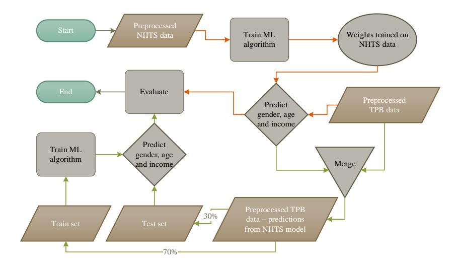
Figure 1. Testing if the national data can be used for regions that lack travel surveys (orange arrows); model fusion for accuracy improvement (green arrows).
The idea of using multiple data sets was to meet the requirement for detailed travel surveys. We aimed to perform the analysis for the Washington metropolitan area (WMA), but we tried different variants to explore the possibilities. First, we used the WMA data to show the validity of our analysis for cases where travel survey data were available. Then, to see what would happen if there were no travel survey data, we used models trained based on the NHTS data to infer the population of WMA. One option was to extract only that part of NHTS that is related to WMA, but this would have reduced our sample size and impacted our model. The third approach was to use both the TPB and the NHTS data. The whole process is depicted in Figure 1.
Model training and prediction
As mentioned previously, we aimed to estimate the travelers' age, gender, and income based on their travel patterns. We used different ML models for this purpose. ML models have been proven to be either well-performing or better than conventional methods; in addition, they are decent choices for detecting complex travel behavior patterns, since they are more flexible and free of assumptions (Koushik, Manoj & Nezamuddin, 2020). The data set prepared in the previous section was used to predict socioeconomic characteristics using deep learning and gradient
boosting models. Some conventional machine learning models were also included for the sake of comparison, namely SVM, Decision Tree, Random Forest, KNN, and Logistic Regression. Age and income prediction were represented as a classification problem, and gender was formulated as a regression problem.
Deep learning. After the study conducted by (Krizhevsky, Sutskever & Hinton, 2012), deep learning models started to gain popularity, as these models far surpassed the other architectures proposed in the Imagenet competition (Russakovsky et al., 2015). Since then these models have been widely adopted not only for image classification purposes but all across the board for academic and practical applications. They offer the opportunity to go wider and deeper in neural networks, which would most likely make stronger models, especially in the context of big data. In addition, similar studies to this paper also made use of such models, which sometimes proved to be the best choice. As such, a deep feed-forward neural network, and two convolutional neural networks (1D and 2D) were included in the modeling process in the hope that these models could exploit the abundance of data and pick up complex travel patterns among different socioeconomic groups.
Gradient boost. Gradient boosting is an ML technique that combines weak learners to create a model with much more robust prediction capabilities. A boosting model starts by training a base model (for example, a decision tree or linear regression). Then a second model is developed that focuses on predicting when the first model performs poorly. This reinforcement process is repeated many times. Each consecutive model tries to correct the shortcomings of the reinforced set by combining all the previous models. This technique relies on the theory that the next best model adjusts the results to minimize the overall prediction error when combined with the previous models. As Gradient Boosting models have shown some promise in recent years, in this study, we used AdaBoost (Hastie, Rosset, Zhu & Zou, 2009), XGBoost (Chen & Guestrin, 2016), LightGBM (Ke et al., 2017), and CatBoost (Prokhorenkova, Gusev, Vorobev, Dorogush & Gulin, 2017). However, CatBoost was picked for further experimentation and hyper-parameter tuning as it yielded the most accurate initial prediction performances.
Bayesian updating. It is possible to improve/update the ML predicted probabilities of the socioeconomic characteristics by employing Bayesian updating. Bayesian updating, also known as Bayesian inference, is a statistical inference method based on the Bayesian theorem that updates the probability of a hypothesis when more information is available. As mentioned in the data section, we also used a synthetic population of the Washington metropolitan area in 2007. There were 3,722 traffic analysis zones (TAZ) in the synthetic data, each with a different income, age, and gender distribution. Therefore, it was possible to update the probabilities estimated by the model based on the residence location of the trip maker. The Bayesian updating formula used was as follows:
\[P(M|E) = \frac{P(E|M)}{\sum_{n} P(E|M_n) P(M_n)} \cdot P(M)\] (1)
where P(M) is the prior probability based on the synthetic population, P(E│M) is the likelihood estimated by the model, and P(M│E) is the posterior probability. We used Bayesian updating for the income groups, as it did not really make much sense to use it for gender (the prior probability of gender is not expected to vary much from 50%).
Results and Discussion
This paper used travel behavior patterns to infer the travelers' gender, age, and income. After the prediction phase, we used Bayesian updating for the Washington metropolitan area to improve the income prediction probabilities based on a synthetic population. This section reports and discusses these outputs. First, the performance of the models trained on the TPB data is reported, then the outcome of Bayesian inference for updating the income levels is discussed. Finally, these results are compared with the models that were trained using the NHTS data.
As can be seen in Table 5, generally, Gradient Boosting had the highest accuracy figures for all predicted characteristics, while the conventional machine learning methods performed very poorly, except for Random Forest. Interestingly, the deep learning algorithms did not live up to their high-performing reputation in our case, showing inferior performance compared to the Gradient Boosting methods. Regarding gender prediction, all the deep learning methods as well as Random Forest and LightGBM showed a moderate accuracy of around 60%. This figure was followed by the other Gradient Boosting methods, whose accuracy was up to 61.93%. This was the highest accuracy for gender prediction, which was obtained by CatBoost but the number was only slightly higher than that of AdaBoost (at 61.89%).
Turning to income predictions, again, Catboost produced the most accurate results at 51.34%, followed closely by Random Forest, LightGBM, and Neural Network at approximately 51.23%. CatBoost was the top-performing model for age prediction as well (at 46.41%).
Table 5. Prediction accuracy comparison among different ML models for gender, income, and age on TPB data
| Method | Model | Gender | Income | age | |
|---|---|---|---|---|---|
| Conventional | Machine | KNN | 52.03% | 39.29% | 32.23% |
| Learning | Decision Tree | 53.54% | 42.10% | 34.55% | |
| Logistic Regression | 57.78% | 47.55% | 40.53% | ||
| SVM | 58.36% | 46.58% | 40.40% | ||
| Random Forest | 60.01% | 51.23% | 43.57% | ||
| Gradient | Boosting | AdaBoost | 61.89% | 49.93% | 44.48% |
| Methods | XGBoost | 61.19% | 51.10% | 45.67% | |
| LightGBM | 60.17 | 51.22 | 45.47 | ||
| CatBoost | 61.93% | 51.34% | 46.41% | ||
| Deep Learning | Neural Network | 60.76 | 51.24% | 44.94% | |
| Convolutional 2D | 60.2% | 49.76% | 43.64% | ||
| Convolutional 1D | 60.05% | 48.98% | 42.28% |
Income was classified into three groups, low (less than $50,000), middle ($50,000 to $100,000), and high (more than $100,000). As shown in Table 6, recall and precision were higher for the $100,000 income category (86.54% and 53.45% respectively), which is not surprising given the high average income in the Washington metropolitan area.
| Estimate | Total | Recall | |||
|---|---|---|---|---|---|
| Actual | <$50,000 | $50,000-100,000 | >100,000$ | ||
| <$50,000 | 225 | 189 | 522 | 936 | 24.03% |
| $50,000- | 124 | 311 | 1550 | 1985 | 15.66% |
| 100,000 | |||||
| >$100,000 | 82 | 288 | 2380 | 2750 | 86.54% |
| Precision | 52.20% | 39.46% | 53.45% | 51.34% |
Table 6. CatBoost confusion matrix for income (TPB)
After calculating the mean income distribution for each TAZ from the synthetic data and applying Bayesian inference to update the income probabilities estimated by the model, the income prediction accuracy of CatBoost increased by 3.3%, from 51.34% (Table 6) to 54.64%. This was a notable improvement, proving that the Bayesian updating is beneficial for this type of analysis.
The predictions for the four age groups showed that the oldest age group (60 and older) was almost always better estimated than the other age groups, while the 40- to 50-year age group had the least correct true positives. People aged 18 to 40 were also predicted fairly accurately (at 67.01% of recall) (Table 7).
| Estimate | Total | Recall | ||||
|---|---|---|---|---|---|---|
| Actual | 18-40 | 40-50 | 50-60 | +60 | ||
| 18-40 | 1215 | 138 | 240 | 220 | 1813 | 67.01% |
| 40-50 | 677 | 150 | 257 | 150 | 1234 | 12.15% |
| 50-60 | 497 | 88 | 409 | 315 | 1309 | 31.24% |
| +60 | 251 | 28 | 178 | 858 | 1315 | 65.24% |
| Precision | 46.02% | 37.12% | 37.73% | 55.60% | 46.41% |
Table 7. CatBoost confusion matrix for age (TPB)
Looking at the gender prediction confusion matrix (Table 8), females were generally better identified by the algorithm. This can be attributed to the higher frequency of female samples in the data, as previously discussed, which is also shown in Table 1.
Table 8. CatBoost confusion matrix for gender (TPB)
| Estimate | Total | Recall | ||
|---|---|---|---|---|
| Actual | Male | Female | ||
| Male | 573 | 605 | 1178 | 48.64% |
| Female | 366 | 1,007 | 1373 | 73.34% |
| Precision | 61.02% | 62.46% | 61.93% |
A summary of the results for the different data sets and approaches is reported in Table 9. Overall, the accuracy of age and gender predictions in this study was better in the models trained with the NHTS data. These models were able to infer gender nearly 3% and age approximately 7% better than the one that was trained with the TBP data. Despite this advantage, the income accuracy of the TPB model was better than that trained by the NHTS data. Therefore, it can be inferred that more samples result in improvement in age and gender prediction, but income is very much influenced by local conditions.
| Gender | Age | Income | |
|---|---|---|---|
| NHTS | 64.2% | 53.68% | 50.23% |
| TPB | 61.93% | 46.41% | 51.34% |
| NHTS+TPB | 63.23% | 45.68% | 51.41% |
Table 9. CatBoost accuracy results summary
Table 10 shows ROC and Cohen's kappa score for the CatBoost model trained in this study. Cohen's kappa income score for TPB data did not agree with the accuracy. Income yielded higher accuracy with the TPB data, but Cohen's cappa score had a higher value with the NHTS data .
Data ROC score Cohen's kappa score Gender Gender Age Income NHTS 0.69 0.2647 0.3397 0.2071 TPB 0.6564 0.2230 0.2643 0.1295
Table 10. ROC and Cohen's kappa score (CatBoost)
Assuming that TPB as a regional data set is a subset of national data (NHTS), the NN model was trained on the NHTS as the training data and was validated on the TPB data. This experiment was conducted to check whether the NHTS data set (national data) is a suitable candidate for model training when an area does not have regional travel survey data. Surprisingly, this resulted in very low validation accuracies, proving this technique is not a viable option. The reasons for this low performance may be threefold: 1) although the data sets are both survey data, the collection year and collection methodology differ to some extent; 2) the travel patterns and socioeconomic characteristics of individuals strongly depend on local factors; 3) socioeconomic distribution varies greatly, to the point where data imbalance causes highly biased predictions.
In an attempt to improve accuracy, we trained the CatBoost model on the NHTS data and used the weights from this model to predict the socioeconomic characteristics of samples from the TPB data (ensemble modeling). Having added the prediction probabilities as new features to the TPB data, a second model was trained. After evaluation, the results indicated that while gender prediction accuracy experienced a significant accuracy increase of 1.3%, the age-group estimation accuracy decreased marginally. In addition, income prediction accuracy also declined, reminding us of the distribution variance of income groups between the Washington metropolitan area and the US as a whole.
The proposed method addresses the problem of linking passively collected mobility data to socioeconomic characteristics without violating privacy. The trained models are expected to be deployed on a stream of crowd-based big mobility data, processing the raw data into travel patterns and then linking the patterns to the most probable socioeconomic characteristics of the travelers. The output can be leveraged for developing new travel demand forecasting models as well as validating existing ones. The same data exists in travel and activity surveys that are collected periodically, but these periods tend to be very long because the collection process is lengthy and expensive. There is much missing information lost between these long gaps, which can be continuously inferred using the proposed method. Thus, the model can save costs for transportation agencies. It can derive key socioeconomic information (age, gender, and income) with developing the proposed model for the region of interest as the initial cost. Although this model can replace traditional surveys in essential information on travel demand, more exploration needs to be done before we can utilize big data as replacement for survey data in other transportation applications.
Despite our best efforts to perform a well-designed study, there were a number of limitations. First, the survey data used for modeling comprised individuals filling their travel diaries for a single day. More measures of travel data for each individual may improve the results, since it will present more travel behavior variability for each socioeconomic group, which could translate into more robust ML models. Second, even though survey data was used to map travel patterns to socioeconomic characteristics, we had to consider the limitations imposed by crowd-based data (e.g. mobile data) for application purposes. This means trip features that were not extractable from these data were not included. For instance, from continuous GPS trajectory data, it is possible to extract home and work locations, and the information pertaining to these locations. However, a wide range of other locations and the purpose of taking a trip to those places are not easily, or at all, possible to extract – at least not in the near future – such as non-mandatory trip purposes: recreation, meal, religion, visiting relatives, etc. Third, the model was developed using the travel data collected for weekdays only. To have a clear picture of travel behavior variability, including data from both weekdays and weekends seems to be helpful. But again, as the purposes of trips conducted on weekends tend to be mainly of the non-mandatory type, they may not be easy to infer from crowd-based data. Yet, they are essential to provide a holistic view of individuals' travel patterns to the pattern recognition algorithm.
Conclusion
In the era of big data, there is a huge interest in using big data as an alternative to travel survey data. However, most forecasting models need socioeconomic variables to make predictions. As the crowd-based data do not contain socioeconomic attributes of individuals, we need to somehow infer them from the data. In this study, we used ML models to infer the socioeconomic characteristics of trip makers based on their travel patterns. It was hypothesized and proven that travel-activity behavior patterns hinge upon socioeconomic characteristics. We preprocessed and analyzed two survey data sets, NHTS 2009 and TBP 2007-2008, and investigated the models' accuracy in inferring socioeconomic characteristics. We used the two data setsto analyze the local effect and investigate the possibility of using NHTS data in cases where travel survey data are unavailable. We used different ML algorithms. The results from these two algorithms were compared on both data sets. CatBoost was proven to outperform all the other models.
Bayesian updating was then used to improve the income prediction of the model based on synthetic population data from the Washington metropolitan area. As a result, the model accuracy was improved by 3%. Since the income distribution in each region is different, the income distribution is more dependent on the region; thus, it is advisable to train income models on regional data rather than national data. Finally, the best age and gender prediction accuracy was obtained from CatBoost using the NHTS data (gender 64.2% and age 53.68%) and the best income accuracy was obtained from training the CatBoost model using the TPB data and then updating the prediction probabilities using the synthetic population data (54.64%).
The correlation results of the trained models can be applied to crowd-based mobility data, for example mobile data or GPS tracking data, to make them an asset in travel demand forecasting. Whereas before, the urban planning process was followed in a one-way manner, from socioeconomic characteristics to travel demand, now, thanks to big data and machine learning, we are able to reverse the process to our advantage.
Future studies can test longer periods of travel data, include travel data of both weekends and weekdays, and endeavor to design procedures to infer more travel destinations from crowd-based data than home, work, and shops. Additionally, future work should include the mode of transport in the model as it is affected by socioeconomic characteristics (Ko, Lee & Byun, 2019) and can be inferred from crowd-based data (Li et al., 2020). Future research may also evaluate the proposed model with more recent data, such as the NHTS 2017 data, using the evidence offered in the present paper. Machine learning models are often referred to as 'black box' processes because they provide a solution or make a judgment without providing a way to understand the internal process. Future studies could employ interpretable machine learning algorithms to analyze the mechanism with which the models relate mobility patterns to socioeconomics. Finally, predicting the employment status of individuals is another direction for future work.
Statements and Declarations
Data and Code Availability: NHTS is an open-source data set available on the FHWA website, and TPB is accessible upon request from MWCOG. The Python implementation used in this study is available as a Github repository.
Conflict of Interest: The authors declare that there are no conflicts of interest regarding the publication of this paper.
Funding: The authors received no financial support for the research, authorship, and/or publication of this article.